Things you need to know about Graph Algorithms
 Fatima Jannet
Table of contents

Let's start learning about Graph Algorithms!
Graph Algorithm
A graph is a nonlinear data structure consisting of finite sets of Vertices (nodes) and a set of Edges which connect a pair of nodes.
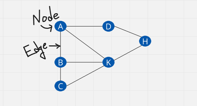
Here, circular objects are the vertices, the lines are the edges. It similar with tree data structure for having connected nodes. Although tree can't make a circular path like graph algo.
Why graph?
Graphs are used to solve many real life problems. They are mostly used in representing networks, i.e. flight paths between cities, telephone network, circuit network etc. Graphs are also used in social networks like Facebook, LinkedIn.
Graph Terminologies
Vertices (vertex): Vertices are the node of a graph
Edge: The edge is the line that connects pairs of vertices
Unweighted graph: A graph which does not have a weight associated with any edge
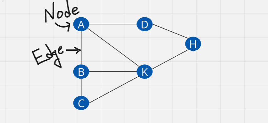
Weighted graph: A graph which has a weight associated with any edge.
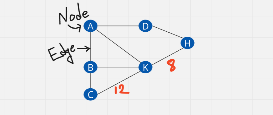
Undirected graph: In case, the edges of the graph have no direction.
Directed graph: Directions are associated
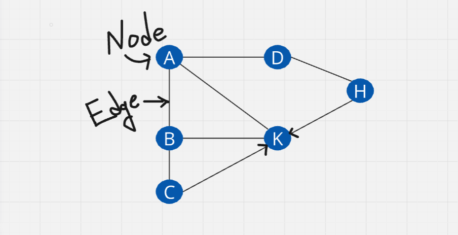
Here, you can go from C to K, but not K to C
Cyclic graph: A graph that has at least one loop
Acyclic graph: A graph with no loop
Tree: It is a special case of directed acyclic graph
Types of Graph
Graph has two categories:
Directed
Weighted
Positive
Negative
Unweighted
Undirected
Weighted
Positive
Negative
Unweighted
As you can see, we have six types of graphs over here. Now let's learn them
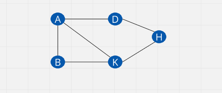
Unweighted - Undirected : Access to the both ways
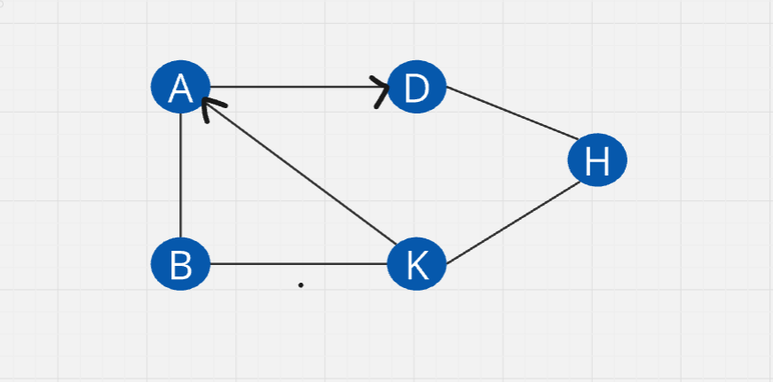
Unweighted - Directed : Access to the directed way only (one way traffic)
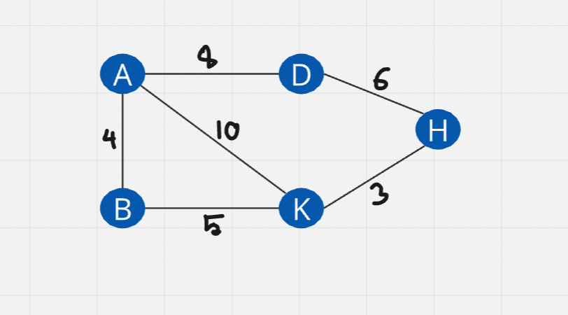
Positive-weighted-undirected :
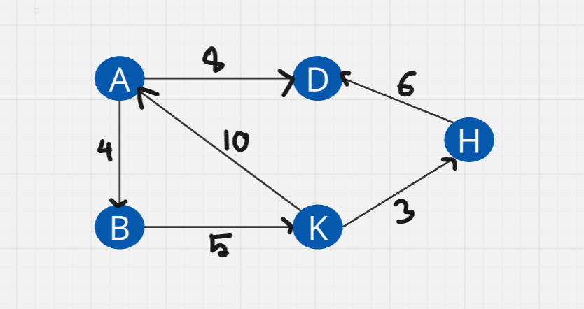
Positive-weighted-directed :
Negative - weighted - undirected :
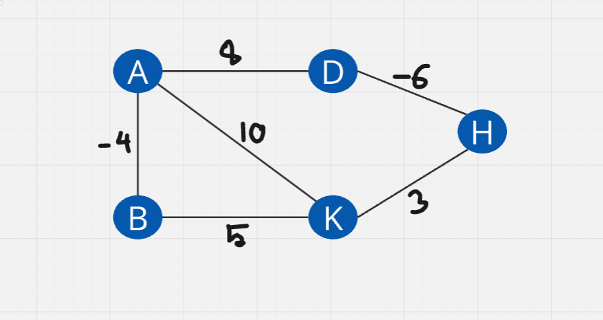
Negative - weighted - Directed:
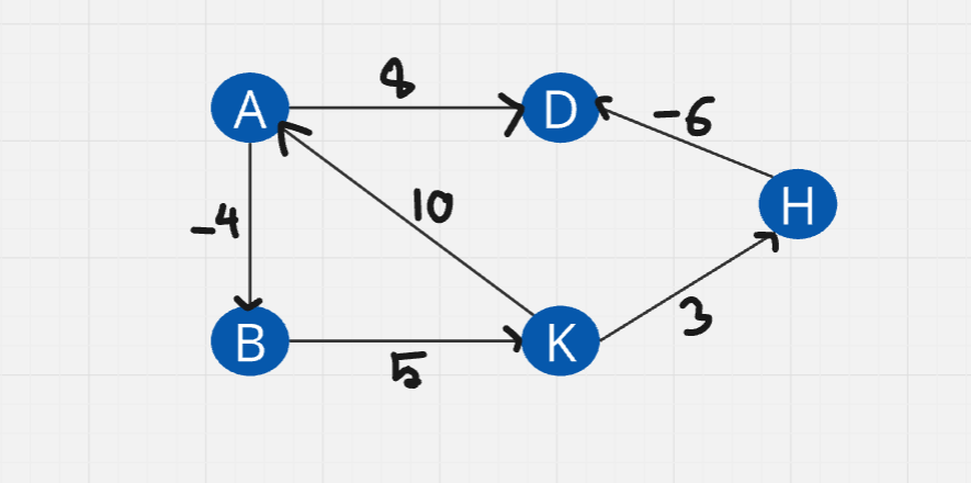
Graph representation
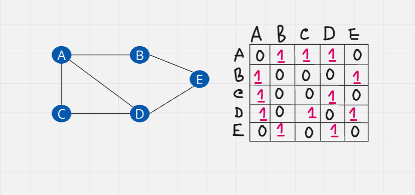
The first way to represent graph is using adjacency matrix.
Adjacency matrix: It is a sq matrix or, a 2D array. The elements of the matrix indicate whether pairs of vertices are adjacent or not in the graph
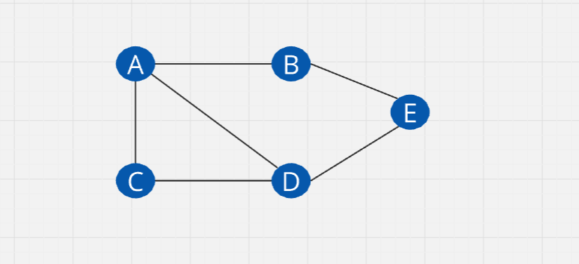
As you can see, there are 5 elements. So we will create a two-dimensional array 5x5, all the elements will be initialized to zero.
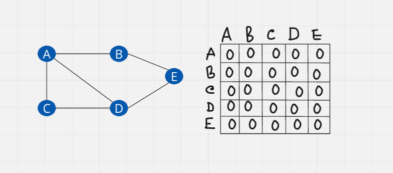
We will change the values from zero to one based on their connection. This matrix represents the path perfectively. From A to B, there's a connection so there's a one for them. Keep doing the process.
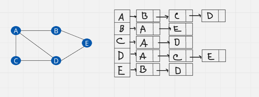
Adjacency List: It is a collection of unordered list used to represent a graph. Each list describes the set of neighbors of a vertex in the graph.
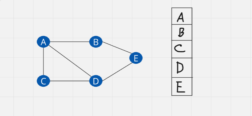
In this case, instead of creating a 2D matrix, we will use 1Darray with the size of five. After that, we will initialize all vertices to the array. Then we will create linked list based on connections (edges)
Which one you should use?
If the graph is a complete graph or almost complete graph, then you should use adjacency matrix. On the other hand, if the number of edges are few, you should use adjacency list.
Create graph using Python
You have guessed we need dictionary implements.
class Graph:
    def __init__(self, gdict=None):
        if gdict is None:
            gdict = {}
        self.gdict = gdict
    def addEdge(self, vertex, edge):
        self.gdict[vertex].append(edge)

customDict = { "a" : ["b", "c"],
                "b" : ["a", "d", "e"],
                "c" : ["a", "e"],
                "d" : ["b", "e", "f"],
                "e" : ["d", "f", "c"],
                "f" : ["d", "e"]
             }
graph = Graph(customDict)
graph.addEdge("e", "c")
print(graph.gdict)
print(graph.gdict["e"])
Create graph using Python - Add Vertex
class Graph:
    def __init__(self):
        self.adjacency_list = {}

    def add_vertex(self, vertex):
        if vertex not in self.addjacency_list.keys():
            self.adjacency_list[vertex] = []
            return True
        return False

    def print_graph(self):
        for vertex in self.adjacency_list:
            print(vertex, ":", self.adjacency_list[vertex])
custom_graph = Graph()
custom_graph.add_vertex("A")
custom_graph.print_graph()
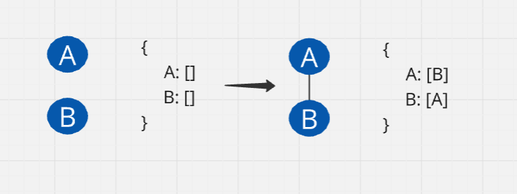
Add edge
Visualization:
class Graph:
    def __init__(self):
        self.adjacency_list = {}

    def add_vertex(self, vertex):
        if vertex not in self.addjacency_list.keys():
            self.adjacency_list[vertex] = []
            return True
        return False

    def print_graph(self):
        for vertex in self.adjacency_list:
            print(vertex, ":", self.adjacency_list[vertex])

    def add_edge(self, vertex1, vertex2):
        if vertex1 in self.adjacency_list.keys() and vertex2 in self.adjacency_list.keys()
            self.adjacency_list[vertex1].append(vertex2)
            self.adjacency_list[vertex2].append(vertex1)
            return True
        return False


custom_graph = Graph()
custom_graph.add_vertex("A")
custom_graph.add_vertex("B")
custom_graph.add_edge("A","B")
custom_graph.print_graph()
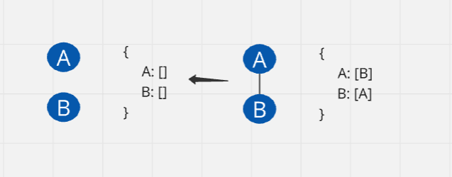
Remove Edge
class Graph:
    def __init__(self):
        self.adjacency_list = {}

    def add_vertex(self, vertex):
        if vertex not in self.addjacency_list.keys():
            self.adjacency_list[vertex] = []
            return True
        return False

    def print_graph(self):
        for vertex in self.adjacency_list:
            print(vertex, ":", self.adjacency_list[vertex])

    def add_edge(self, vertex1, vertex2):
        if vertex1 in self.adjacency_list.keys() and vertex2 in self.adjacency_list.keys() :
            self.adjacency_list[vertex1].append(vertex2)
            self.adjacency_list[vertex2].append(vertex1)
            return True
        return False

    def remove_edge(self, vertex1, vertex2):
        if vertex1 in self.adjacency_list.keys() and vertex2 in self.adjacency_list.keys() :
            try:
                self.adjacency_list[vertex1].remove(vertex2)
                self.adjacency_list[vertex2].remove(vertex1)
            except ValueError:
                pass
            return True
        return False

custom_graph = Graph()
custom_graph.add_vertex("A")
custom_graph.add_vertex("B")
custom_graph.add_vertex("C")
custom_graph.add_vertex("D")
custom_graph.add_edge("A","B")
custom_graph.add_edge("A","C")
custom_graph.add_edge("B","C")
custom_graph.print_graph()
custom_graph.remove_edge("A","D")
To avoid value error, I've added try, except block in the code.
Remove vertex
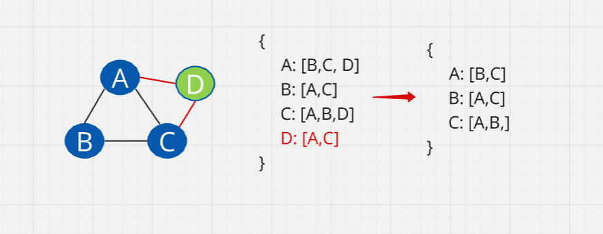
When removing a vertex, it will be removed along with its edges.
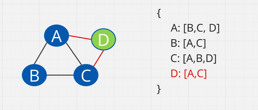
To delete an edge, we check the list of edges. We loop through the list to find the vertices in the adjacency list. First, we find vertex A and delete D from A's values. Next, we find C and delete D from C's values. Finally, we go to D and delete it. This is very efficient even if there were thousands of elements.
Time to implement:
class Graph:
    def __init__(self):
        self.adjacency_list = {}

    def add_vertex(self, vertex):
        if vertex not in self.addjacency_list.keys():
            self.adjacency_list[vertex] = []
            return True
        return False

    def print_graph(self):
        for vertex in self.adjacency_list:
            print(vertex, ":", self.adjacency_list[vertex])

    def add_edge(self, vertex1, vertex2):
        if vertex1 in self.adjacency_list.keys() and vertex2 in self.adjacency_list.keys() :
            self.adjacency_list[vertex1].append(vertex2)
            self.adjacency_list[vertex2].append(vertex1)
            return True
        return False

    def remove_edge(self, vertex1, vertex2):
        if vertex1 in self.adjacency_list.keys() and vertex2 in self.adjacency_list.keys() :
            try:
                self.adjacency_list[vertex1].remove(vertex2)
                self.adjacency_list[vertex2].remove(vertex1)
            except ValueError:
                pass
            return True
        return False

    def remove_vertex(self, vertex):
        if vertex in self.adjacency_list.keys():
            for other_vertex in self.adjacency_list[vertex]:
                self.adjacency_list[other_vertex].remove[vertex]
            del self.adjacency_list[vertex]
            return True
        return False

custom_graph = Graph()
custom_graph.add_vertex("A")
custom_graph.add_vertex("B")
custom_graph.add_vertex("C")
custom_graph.add_vertex("D")
custom_graph.add_edge("A","B")
custom_graph.add_edge("A","C")
custom_graph.add_edge("A","D")
custom_graph.add_edge("B","C")
custom_graph.add_edge("C","D")
custom_graph.print_graph()
custom_graph.remove_vertex("D")
print("after removing")
custom_graph.print_graph()
Graph Traversal
Graph traversal means visiting each vertex of the graph. The question is, which node we be visited after current node. Graph can be traversed in two ways 1) Breadth First Search and 2) Depth First Search
Graph Traversal - Breadth First Search (BFS)
It starts at some arbitrary node of the graph and explore the neighbor nodes first before moving to the next level.
Visualization:
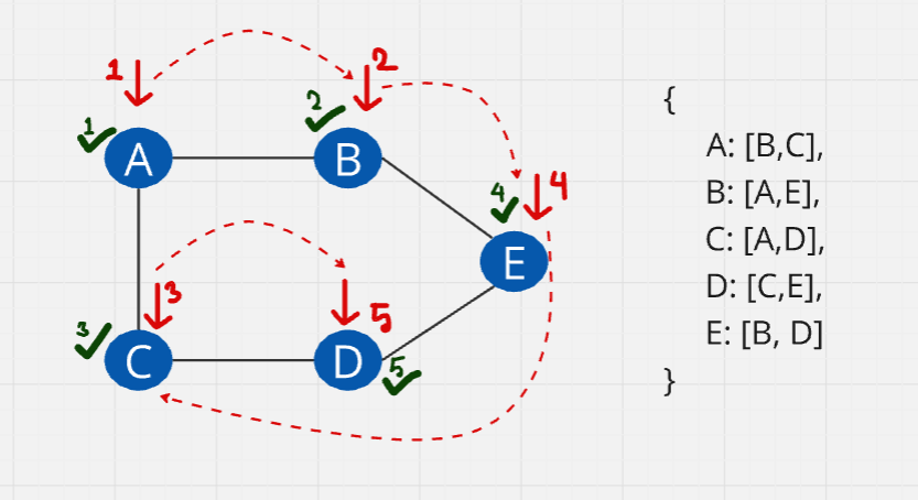
Let's start from A. After visiting A, we mark it as visited and move to its adjacent vertices, B and C. We then mark B and C as visited. Next, we go to B's adjacent vertices, A and E. Since A is already visited, we visit E and mark it as visited. We continue this process.
#from collections import dequeue
def bfs(self, vertex):
    visited = set()
    visited.add(vertex)
    queue = [vertex]
    #queue = dequeue([vertex])
    while queue:   #O(V)
        current_vertex = queue.pop(0) #O(N)
       #current_vertex = queue.popleft(0) #O(V)
        print(current_vertex)
        for adjacent_vertex in self.adjacency_list[current_vertex]: #O(E)
            if adjacent_vertex not in visited:
                visited.add(adjacent_vertex)
                queue.append(adjacent_vertex)
#memory :
#visited = {A,B,C,E,D}
#queue = []
#current_vertex = D

custom_graph = Graph()
custom_graph.add_vertex("A")
custom_graph.add_vertex("B")
custom_graph.add_vertex("C")
custom_graph.add_vertex("D")
custom_graph.add_edge("A","B")
custom_graph.add_edge("A","C")
custom_graph.add_edge("A","D")
custom_graph.add_edge("B","C")
custom_graph.add_edge("C","D")
custom_graph.print_graph()
custom_graph.bfs("A")
Initialization:
visited = set(): This creates a set to keep track of all visited vertices, ensuring that each vertex is visited only once.visited.add(vertex): The starting vertex is added to the visited set.queue = [vertex]: A queue is initialized with the starting vertex. BFS uses a queue to explore the graph level by level.
Specific State:
visited = {A, B, C, E, D}queue = []current_vertex = D
At this point:
The
visitedset includes verticesA, B, C, E, D, meaning they have all been visited.The
queueis empty, indicating that no more vertices are left to explore.The
current_vertexisD, which was the last vertex processed.
We use set instead of list because set gives us O91) time complexity, where list give O(n) time complexity. On he other hand. set aquatically handles uniqueness.
Time complexity: O(V+E) , Space complexity: O(V) (V is the number of vertices, E is the number of edges .You can use dequeue to improve complexity.)
Graph Traversal - Depth First Search (DFS)
Let's start from A. After visiting A, we mark it as visited and move to its first adjacent vertex, B. We then mark B as visited and continue to B's first unvisited adjacent vertex, which is E. From E, we move to its adjacent vertex D, marking it as visited. Finally, we visit D's adjacent vertex C and mark it as visited. Since C has no unvisited neighbors, we backtrack to D, then to E, and so on, until we return to A, ensuring all vertices have been visited.
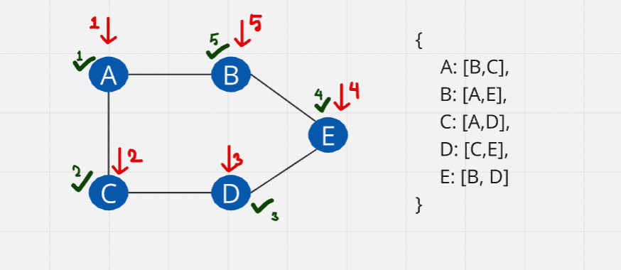
We create a visited set to keep track of all the visited elements. The first vertex is placed in the stack.
def dfs(self, vertex):
    visited = set()
    stack = [vertex]
    while stack: #O(V)
        current_vertex = stack.pop()
        if current_vertex not in visited:
             print(current_vertex)
             visited.add(current_vertex)
        for adjacent_vertex in self.adjacency_list[current_vertex]: #O(E)
            if adjacency_vertex not in visited:
                stack.append(adjacent_vertex)

custom_graph = Graph()
custom_graph.add_vertex("A")
custom_graph.add_vertex("B")
custom_graph.add_vertex("C")
custom_graph.add_vertex("D")
custom_graph.add_edge("A","B")
custom_graph.add_edge("A","C")
custom_graph.add_edge("A","D")
custom_graph.add_edge("B","C")
custom_graph.add_edge("C","D")
custom_graph.print_graph()
custom_graph.dfs("A")
Time complexity: O(V+E) , Space complexity: O(V)
BFS vs DFS
BFS (Breadth-First Search):
Traversal Method: BFS explores the graph level by level, visiting all neighbors of a node before moving to the next level.
Data Structure Used: BFS uses a queue to process vertices in the order they are discovered.
Use Cases: BFS is great for finding the shortest path in unweighted graphs and finding the nearest neighbor.
Example: Like ripples in water, BFS explores each ripple before moving outward.
DFS (Depth-First Search):
Traversal Method: DFS explores as far as possible along each branch before backtracking.
Data Structure Used: DFS uses a stack (explicitly or via recursion).
Use Cases: Useful for pathfinding, topological sorting, and cycle detection.
Example: Like navigating a maze—follow one path until you hit a wall, then backtrack.
Key Differences:
Order of Exploration: BFS explores neighbors first, while DFS goes deep along a path before backtracking.
Data Structure: BFS uses a queue, while DFS uses a stack or recursion.
Pathfinding: BFS finds the shortest path in unweighted graphs; DFS might not.
Complexity: Both have a time complexity of O(V + E), where V is vertices and E is edges.
When to Use:
BFS: For finding the shortest path or exploring all possibilities level by level.
DFS: For exploring deep paths, checking for cycles, or visiting every vertex systematically.
Understanding the differences between BFS and DFS helps in choosing the right approach based on the problem's requirements.
End.
Subscribe to my newsletter
Read articles from Fatima Jannet directly inside your inbox. Subscribe to the newsletter, and don't miss out.
Written by
