Get Your Data in Shape: The Ultimate Guide to Feature Scaling

I hope you are doing well. Today, we will dive deep into the concept of feature scaling in machine learning. Here are a few questions we will answer throughout this blog post:

• What is feature scaling, and why is it necessary?

• What are the different techniques used for feature scaling?

• When should each technique be used?

Note: Along with the theoretical understanding, we will also go over Python programs to solidify our practical implementation skills. So, without any further ado, let's get started.

What is feature scaling ?

Feature scaling is a data preprocessing technique that falls under the broader term of feature engineering. The main idea behind this technique is to ensure that all the features (columns) in our data are brought to the same scale. But why is it so important to bring the features to a common scale? What happens if we don't do it?

There are two reasons that, in my opinion, are enough to convince you why we need to do feature scaling.

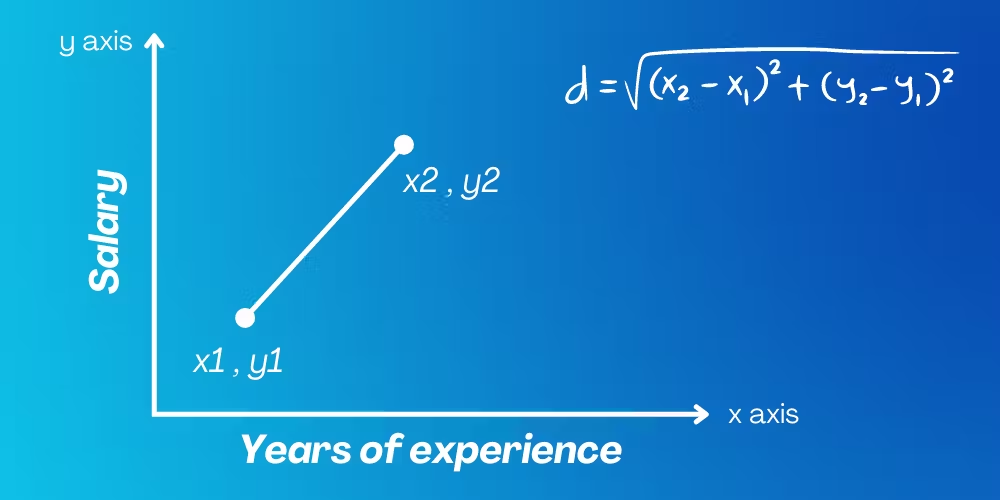
• Reason 1: Without feature scaling, the performance of distance-based algorithms will degrade. These algorithms rely on distance metrics like Euclidean distance. If the features are not on the same scale, one feature will overpower the other, leading to unstable or incorrect results.

  

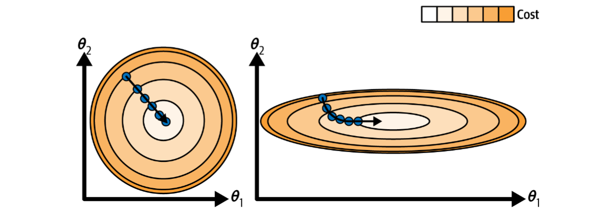
• Reason 2: It has been observed experimentally that when feature values are scaled to a common scale, the convergence speed of optimization algorithms like Gradient Descent improves. This leads to better and faster training.

  

What are the various techniques we can use for feature scaling?

There are basically three main feature scaling techniques. Let's take a look at each of them along with their mathematical formulas and code.

Standardization ( Z score normalization )

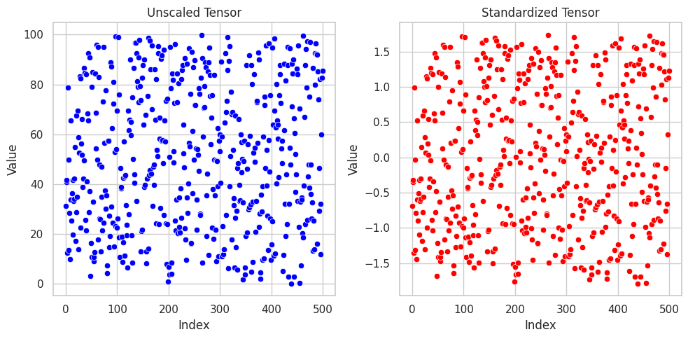
Standardization, also known as z-score normalization, is a feature scaling technique used for mean centering the data. In simple terms, this means that after applying this technique, the mean of the feature values becomes 0 and the standard deviation becomes 1. Mathematically, it is expressed as:

$$z = (x-μ)/σ$$

import torch
from rich import print
import matplotlib.pyplot as plt

def standardize_tensor(tensor):
    """
    Standardizes the given tensor by subtracting the mean and dividing by the standard deviation.

    Parameters:
    tensor (torch.Tensor): The input tensor to be standardized.

    Returns:
    torch.Tensor: The standardized tensor.
    """
    # Ensuring the tensor is of float type
    tensor = tensor.float()

    # Calculating the mean and standard deviation
    mean = torch.mean(tensor)
    std_dev = torch.std(tensor)
    # Standardizing the tensor
    standardized_tensor = (tensor - mean) / std_dev
    return standardized_tensor


# Generating 500 random values uniformly distributed between 0 and 100
unscaled_tensor = torch.rand(500) * 100  

# Standardizing the tensor
standardized_tensor = standardize_tensor(unscaled_tensor)


# Plotting the scatter plot for both the unscaled tensor and the standardized tensor
sns.set(style="whitegrid")
fig, axes = plt.subplots(1, 2, figsize=(10, 5))

# Scatter plot for the unscaled tensor
sns.scatterplot(x=range(len(unscaled_tensor)), y=unscaled_tensor, color='blue', ax=axes[0])
axes[0].set_title('Unscaled Tensor')
axes[0].set_xlabel('Index')
axes[0].set_ylabel('Value')

# Scatter plot for the standardized tensor
sns.scatterplot(x=range(len(standardized_tensor)), y=standardized_tensor, color='red', ax=axes[1])
axes[1].set_title('Standardized Tensor')
axes[1].set_xlabel('Index')
axes[1].set_ylabel('Value')

plt.tight_layout()
plt.show()

Normalization ( Min-Max normalization )

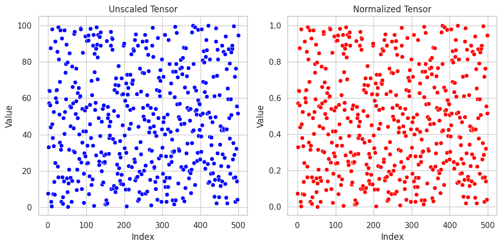
Normalization, also known as min-max normalization, is a feature scaling technique which is used when we want to squeeze the feature values between the range of 0 to 1 (inclusive). Mathematically, it is expressed as:

$$z = (x-x_{min})/(x_{max}-x_{min})$$

import torch
from rich import print
import matplotlib.pyplot as plt
import seaborn as sns

def normalize_tensor(tensor):
    """
    Normalizes the given tensor by scaling its values to a common range, usually between 0 and 1.

    Parameters:
    tensor (torch.Tensor): The input tensor to be normalized.

    Returns:
    torch.Tensor: The normalized tensor.
    """
    # Ensuring the tensor is of float type
    tensor = tensor.float()

    # Calculating the minimum and maximum values
    min_val = torch.min(tensor)
    max_val = torch.max(tensor)
    # Normalizing the tensor
    normalized_tensor = (tensor - min_val) / (max_val - min_val)
    return normalized_tensor


# Generating 500 random values uniformly distributed between 0 and 100
unscaled_tensor = torch.rand(500) * 100  

# Normalizing the tensor
normalized_tensor = normalize_tensor(unscaled_tensor)


# Plotting the scatter plot for both the unscaled tensor and the normalized tensor
sns.set(style="whitegrid")
fig, axes = plt.subplots(1, 2, figsize=(10, 5))

# Scatter plot for the unscaled tensor
sns.scatterplot(x=range(len(unscaled_tensor)), y=unscaled_tensor, color='blue', ax=axes[0])
axes[0].set_title('Unscaled Tensor')
axes[0].set_xlabel('Index')
axes[0].set_ylabel('Value')

# Scatter plot for the normalized tensor
sns.scatterplot(x=range(len(normalized_tensor)), y=normalized_tensor, color='red', ax=axes[1])
axes[1].set_title('Normalized Tensor')
axes[1].set_xlabel('Index')
axes[1].set_ylabel('Value')

plt.tight_layout()
plt.show()

Robust Scaling

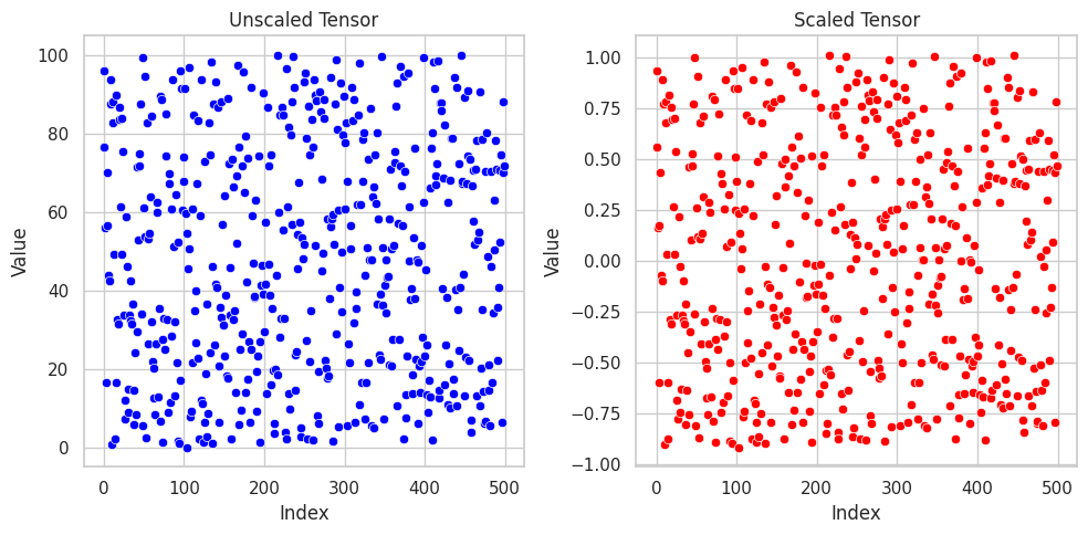
Robust scaling is specifically used to scale data with outliers. This technique uses the median and interquartile range (IQR) instead of the mean and standard deviation for scaling and after the scaling the data is median centered. Mathematically, it is defined as:

$$z = (x-Median(x))/IQR(x)$$

import torch
from rich import print
import matplotlib.pyplot as plt
import seaborn as sns

def robust_scale_tensor(tensor):
    """
    Robustly scales the given tensor by scaling its values to a common range, usually between 0 and 1,
    using the interquartile range (IQR) to handle outliers.

    Parameters:
    tensor (torch.Tensor): The input tensor to be scaled.

    Returns:
    torch.Tensor: The robustly scaled tensor.
    """
    # Ensuring the tensor is of float type
    tensor = tensor.float()

    # Calculating the median and interquartile range (IQR)
    median = torch.median(tensor)
    Q1 = torch.quantile(tensor, 0.25)
    Q3 = torch.quantile(tensor, 0.75)
    IQR = Q3 - Q1

    # Robust scaling the tensor
    scaled_tensor = (tensor - median) / IQR
    return scaled_tensor


# Generating 500 random values uniformly distributed between 0 and 100
unscaled_tensor = torch.rand(500) * 100  

# Robustly scaling the tensor
scaled_tensor = robust_scale_tensor(unscaled_tensor)


# Plotting the scatter plot for both the unscaled tensor and the scaled tensor
sns.set(style="whitegrid")
fig, axes = plt.subplots(1, 2, figsize=(10, 5))

# Scatter plot for the unscaled tensor
sns.scatterplot(x=range(len(unscaled_tensor)), y=unscaled_tensor, color='blue', ax=axes[0])
axes[0].set_title('Unscaled Tensor')
axes[0].set_xlabel('Index')
axes[0].set_ylabel('Value')

# Scatter plot for the scaled tensor
sns.scatterplot(x=range(len(scaled_tensor)), y=scaled_tensor, color='red', ax=axes[1])
axes[1].set_title('Scaled Tensor')
axes[1].set_xlabel('Index')
axes[1].set_ylabel('Value')

plt.tight_layout()
plt.show()

When to use which technique ?

Now that we understand how each technique works, let's discuss practical tips on when to use each one. Follow these guidelines, and you'll never have to second-guess your choice:

• When the data has natural limits:

  • Examples: Age, percentage, or any feature with a natural minimum and maximum value.

  • Scaling Method: Normalization (Min-Max Scaling) is often appropriate because it scales the data to a fixed range (typically [0, 1] or [-1, 1]), which is helpful for features with known bounds.

• When the data does not have natural limits:

  • Examples: Monetary values or any feature that does not have a fixed upper or lower bound.

  • Scaling Method: Standardization (Z-score Scaling) is often used. It transforms the data to have a mean of 0 and a standard deviation of 1, making it more suitable for features with no natural limits and typically helps with convergence in many machine learning algorithms.

• When the data has outliers and does not have natural limits:

  • Examples: Features with extreme values or skewed distributions without clear bounds.

  • Scaling Method: Robust Scaling is recommended. It uses the median and interquartile range (IQR) to scale the data, making it less sensitive to outliers and better suited for features with extreme values or heavy-tailed distributions.

Conclusion

Well done, you’ve made it through the wild world of feature scaling! 🎉 Next time you’re preparing your data for its big debut in a model, think about which scaling method will make it look its best. With the right scaling, your data will be ready to shine, and your models will perform like a charm. By the way, I would love to connect with you, so here are my social links.

• Github

• Linkedin