In this blog we will deeply dive into data and data preprocessing required before using any raw data for training ML model. before going further let's quickly revise what we learned in last blog of this series. We talked about machine learning, type of data used to train model and some libraries available in python for machine learning.

Now let's see how data is gathered and preprocessed and why we need to preprocess our data.

1. Understand your data

Most important part of the creating a model is to have a sound business knowledge of the problem you are trying to solve.

To gather and know about your data you need to do some research.

1. Primary research

   -Ask questions and gather information from the stakeholders

   -If possible take a dry run of problem you are trying to investigate

2. Secondary research

   -Read reports and studies by government agencies, trade associations or other businesses in your industry

   -Go through any previous work and findings related to your problem

Next step should be to use the acquired business knowledge to search for relevant data.

1. Internal Data: Data collected by your organization

   E.g. Usage data, sales data, promotion data or simply your own collected data through google forms etc.

2. External Data: Data acquired from external data sources

   E.g. Census Data, External vendor Data, Scrape data or simply any available dataset

1.2 Raw Data Analysis

Next step should be to understand the data. You should know variable definition and distribution. prepare a Comprehensive data dictionary which includes

• Definition of predictor variables

• Unique identifier of each table (primary key)

• Explanation of values in case of Categorical variables

We are using housing price dataset for further training a model to predict the price of house based on certain properties.The data set contains 506 observations of house prices from different towns. Corresponding to each house price, data of 18 other variables is available on which price is suspected to depend.

The Data dictionary will be like

• price: Value of the house

• crime_rate: Crime rate in that neighborhood

• resid_area: Proportion of residential area in the town

• air_qual: Quality of air in that neighborhood

• room_num: Average number of rooms in houses of that locality

• age: How old is the house construction in years

• dist1: Distance from employment hub 1

• dist2: Distance from employment hub 2

• dist3: Distance from employment hub 3

• dist4: Distance from employment hub 4

• teachers: Number of teachers per thousand population in the town

• poor_prop: Proportion of poor population in the town

• airport: Is there an airport in the city? (Yes/No)

• n_hos_beds: Number of hospital beds per 1000 population in the town

• n_hot_rooms: Number of hotel rooms per 1000 population in the town

• waterbody: What type of natural fresh water source is there in the city (lake/ river/ both/ none)

• rainfall: The yearly average rainfall in centimeters

• bus_ter: Is there a bus terminal in the city? (Yes/No)

• parks: Proportion of land assigned as parks and green areas in the town

As this is raw data it contain some useless data for our model and many more, We will detect all of them in dataset and will take necessary actions.

1.2 Univariate Analysis

Univariate analysis is the simplest form of analyzing data. In simple words, your data has only one variable. It doesn’t deal with causes or relationships (unlike regression) and it’s major purpose is to describe; it takes data, summarizes that data and finds patterns in the data.

Ways to describe patterns found in univariate data

1. Central tendency- Mean, Mode, Median

2. Dispersion- Range, Variance, maximum, minimum, Quartiles (including the interquartile range), and Standard deviation

3. Count /Null count

Now we will see Why and How data is preprocessed, but before that let's import dataset and libraries in our code file. we are using jupyter notebook for all implementations.

Get all codes and dataset uploaded on my GitHub for your reference, click on below link:

code for data preprocessing

# import required libraries
import numpy as np
import pandas as pd
import seaborn as sns

#import data into dataframe
df= pd.read_csv("House_Price.csv", header= 0)
# header=0 beacause the 0th row of csv is header 

# have a look on top 5 rows of data
df.head()

EDD (Extended Data Dictionary)

# shape of dataframe (506,19)
df.shape
# know more about each variable, null count and data type
df.info()
# statistical summary of all numeric variables
df.describe()

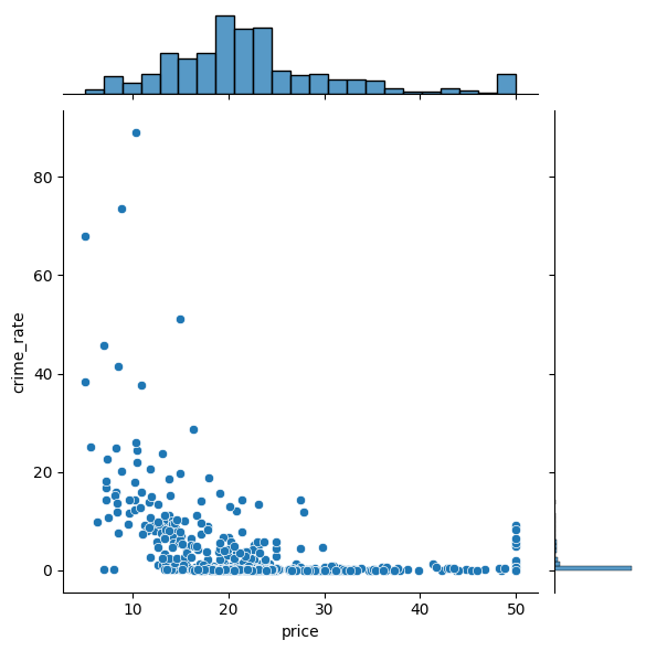
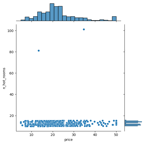
In "crime_rate" and "n_hos_rooms" columns we can see there is large difference between mean value and maximum value. Here the data may be skewed

Analyze the data using scatter plot for such attribute

# we use jointplot method of seaborn library to 
#scatter plot between two variables 
sns.jointplot(y="crime_rate", x="price", data=df)
sns.jointplot(y="n_hot_rooms", x="price",data=df)
sns.jointplot(x="rainfall", y="price", data=df)

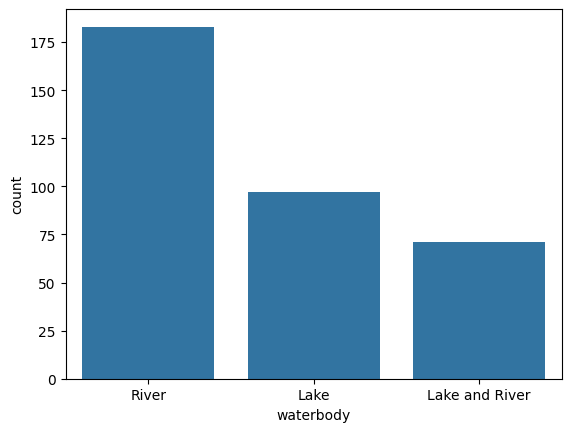
# use countplot to plot categorical variables
sns.countplot(x="airport", data=df)
sns.countplot(x="waterbody", data=df)
sns.countplot(x="bus_ter", data=df)

Skewed Data

Data with outliers

Categorical data

Let's see one by one how the data is preprocessed to get best form of data suitable and efficient to your model.

2. Outlier Treatment

Outlier is a commonly used terminology by analysts and data scientists, Outlier is an observation that appears far away and diverges from an overall pattern in a sample.

Reasons:

• • Data Entry Errors

  • Measurement Error

  • Sampling error etc

Impact : It increases the error variance and reduces the power of statistical tests. below example perfectly explains how outlier make large difference in value of mean, variance and standard deviation.

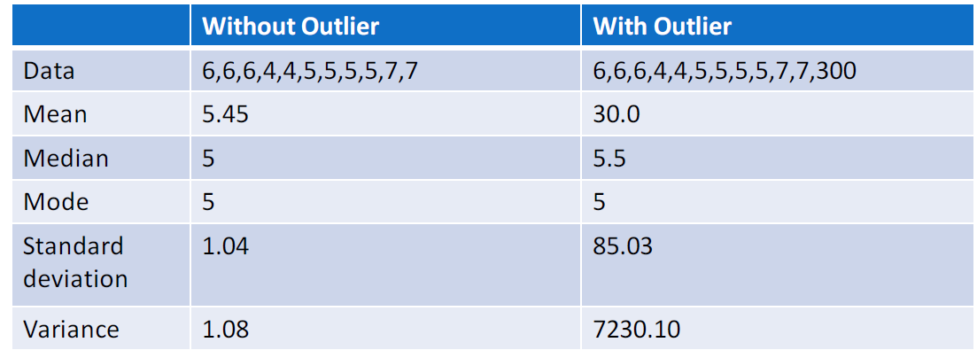
Solution: Detect outliers using EDD and visualization methods such as scatter plot, histogram or box plots then Impute outliers.

There are three method to impute outliers:

2.1 Capping and flooring:

• In this method we find value which is above 99 percentile of data, say P99 and the value which is lower than 1 percentile of data, say P1

• Now replace all values greater than 3*P99 with 3*P99 and replace all values lower than 0.3*P1 with 0.3*P1

• You can use any multiplier instead of 3, as per your business requirement

# find 99 percentile
np.percentile(df['n_hot_rooms'],[99])  #returns array= array([15.39952])
#upper value
uv = np.percentile(df['n_hot_rooms'],[99])[0]  #value at 0th index in returned array
#get outliers
df[(df.n_hot_rooms > uv)] #such rows which has n_hos_room value > upper limit
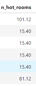
#cap outliers : impute 3*99%le at values greater than uv
df.n_hot_rooms[(df.n_hot_rooms > 3*uv)] = 3 * uv

before imputation:

after imputation:

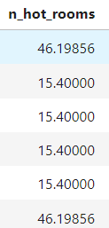
In "n_hot_rooms" outliers were above 99%le of values, but in "rainfall" outliers are below 1%le

lv= np.percentile(df.rainfall,[1])[0] #lower value
df.rainfall[(df.rainfall < 0.3*lv)] = 0.3*lv

2.2 Exponential Smoothing

• Extrapolate curve between P95 to P99 and cap all the values falling outside to the value generated by the curve

• Similarly, extrapolate curve between P5 and P1

• "crime_rate" data is skewed, hence we use exponential smoothing

we will see exponential smoothing in detail in variable transformation part.

2.3 Sigma Approach

• Identify outliers by capturing all the values falling outside 𝝁 ∓ 𝔁𝝈

• You can use any multiplier as x, as per your business requirement

3. Missing Value Imputation

Real-world data often has missing values. Data can have missing values for a number of reasons such as observations that were not recorded and data corruption.

Impact : Handling missing data is important as many machine learning algorithms do not support data with missing values.

Solution:

1. Remove Missing Data:

• Drop Rows: Remove rows with missing values if they are few and don't significantly affect the analysis.

• Drop Columns: Remove columns with too many missing values or if the column is not crucial for analysis.

2. Imputation:

• Mean/Median/Mode Imputation: Replace missing values with the mean, median, or mode of the column (works well for numerical data).

• Forward/Backward Fill: For time-series data, fill missing values with previous (forward fill) or next (backward fill) values.

• Predictive Imputation: Use algorithms like K-Nearest Neighbors (KNN) or regression to predict and fill missing values.

3. Flag and Fill:

• Add a new binary column indicating where data is missing and then fill missing values using one of the above methods.

# look into data to know null values
df.info()
#missing values in h_hos_beds
#sort to see Null values
df.sort_values(by=["n_hos_beds"], na_position="first")

#impute n_hos_beds(numerical variable) with its mean value 
df.n_hos_beds = df.n_hos_beds.fillna(df.n_hos_beds.mean())

4. Noisy Data

Noisy data refers to data that contains errors, random variations, or irrelevant information, which can distort analysis and predictions. It often includes outliers, missing values, or incorrect entries that reduce the data's quality.

To handle noisy data, you can use the following techniques:

1. Binning:

   • First, sort the data and partition it into bins (often equal-frequency).

   • Then apply smoothing techniques:

     • Smooth by bin means: Replace all values in a bin by the mean of the bin.

     • Smooth by bin medians: Replace values with the median of the bin.

     • Smooth by bin boundaries: Replace values near the boundary with the boundary value.

2. Regression:

   • Fit the data to a regression function, like linear or polynomial regression, to smooth the data.

3. Clustering:

   • Group similar data points into clusters and treat points that don’t fit well in any cluster as outliers (noisy data) that can be removed or treated.

4. Combined Computer and Human Inspection:

   • Automatically detect suspicious or outlier values using algorithms, and then allow human inspection to verify and handle them accordingly. This is often used when there’s uncertainty in how to handle detected anomalies.

5.1 Data Transformation

Data transformation involves converting data into a new format, making it more suitable for analysis by mapping old values to new ones.

Need of Normalization?

• Normalization: Needed when data has varying scales and when distance-based models like KNN or clustering are used.

• Standardization: Needed for algorithms that assume normal distribution or when the features have different units.

Types of Normalization:

1. Min-Max Normalization:

   Rescales the data to a specific range, typically [0, 1] or [-1, 1]. It ensures all values are within a common scale.

   

2. Z-Score Normalization (Standardization):

   Rescales data so that it has a mean of 0 and a standard deviation of 1, making the data normally distributed.

   

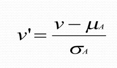
   Useful in machine learning algorithms like SVM, logistic regression that expect normally distributed data.

3. Normalization by Decimal Scaling:

   Moves the decimal point of values in a feature based on the feature's maximum absolute value. If the maximum absolute value is 999, values will be divided by 1000.

   

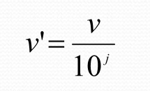
   Example: For values between -999 and 999, dividing by 1000 normalizes the values between -1 and 1.

4. Hierarchy Climbing:

   Replaces low-level values with higher-level concepts from a hierarchy. It helps in generalizing data.

   Example: Instead of using individual ages, group them into ranges like "0-18", "19-35", and "36-60" to capture patterns at a higher level.

Each transformation type serves different purposes, helping you preprocess data for specific models or analysis methods.

Data Discretization

Discretization is the process of transforming continuous numerical data into discrete bins or intervals, making it easier to analyze and suitable for certain types of machine learning models that require or perform better with discrete inputs.

By grouping continuous values into discrete bins, discretization reduces the size and complexity of the data, which can improve computational efficiency.

5.2 Variable Transformation

Before diving into the variable transformation let's understand what is bivariate analysis.

5.2.1 Bivariate Analysis

Bivariate analysis is the simultaneous analysis of two variables (attributes). It explores the concept of relationship between two variables, whether there exists an association and the strength of this association, or whether there are differences between two variables and the significance of these differences.

Scatter Plot:

• Scatter indicates the type (linear or non-linear) and strength of the relationship between two variables

• We will use Scatter plot to transform variables

Correlation:

• Linear correlation quantifies the strength of a linear relationship between two numerical variables.

• When there is no correlation between two variables, there is no tendency for the values of one quantity to increase or decrease with the values of the second quantity.

• Correlation is used to drop Non Usable variables

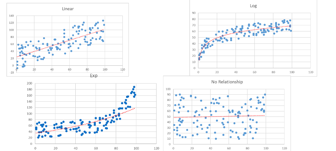
Transform your existing variable to extract more information out of them.

Methods:

• Use Mean/Median of variables conveying similar type of information

• Create ratio variable which are more relevant to business

• Transform variable by taking log, exponential, roots etc.

5.2.2 Variable Transformation

Method 1: In out data dist1, dist2, dist3, dist4 are distance from different employment hubs. They are conveying the similar type of information hence we create a new variable to transform all distances into one.

#add new variable
df["avg_dist"]= (df.dist1+df.dist2+df.dist3+df.dist4)/4
# delete previous variables
del df["dist1"]
del df["dist2"]
del df["dist3"]
del df["dist4"]

Method 2: The plot of 'crime_rate' vs 'price' is logarithmic curve, that is skewed data. Hence instead of taking X (crime_rate) as predictor variable we consider log(X), but log(0) is infinity so we take log(1+X).

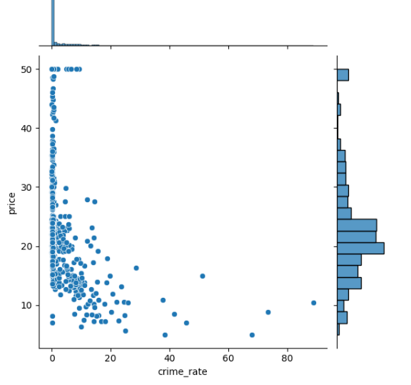
df.crime_rate = np.log(1+df.crime_rate)

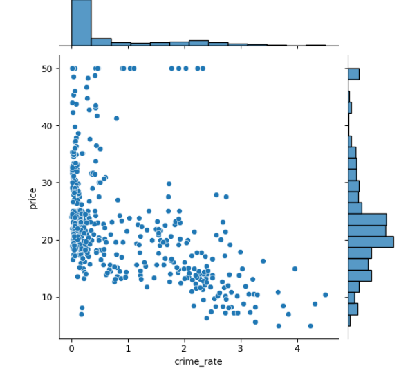
Now the data is somewhat linear.

5.2.3 Non-Usable Data

Identify the non usable variables to reduce the dimension of your dataset. Variable is non usable if

• Variables with single unique value

• Variables with low fill rate

• Variables with regulatory issue

• Variable with no business sense

If you observe the count plot of "bus_ter" it has only one value i.e. YES, Hence we delete such variable

del df['bus_ter']

5.2.4 Encoding - Create Dummy Variables

When working with categorical data in machine learning, many algorithms require numerical inputs, so converting categorical values into numerical representations is essential. This can be done using various encoding methods, each suitable for different types of data:

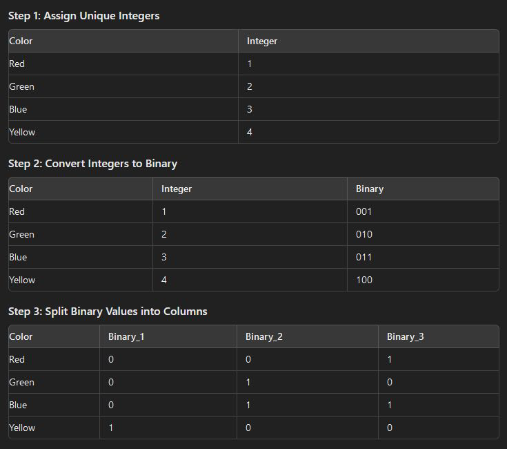
1. Label Encoding: if data values for specific features are ordinal type then label encoding is used. In this, order is important hence the ordered numbering is assigned for data values. e.g. passing grades are given like distinction, first-class, second higher class, second class and pass class. Then in label encoding grades are represented as 0 to 4 respectively.

2. One hot Encoding: this type of encoding is used when categorical data is of type nominal, where there is no ordering. In this encoding for each category one variable is created and if the dataset is of that category then the value 1 is assigned if not then 0 is assigned.

   

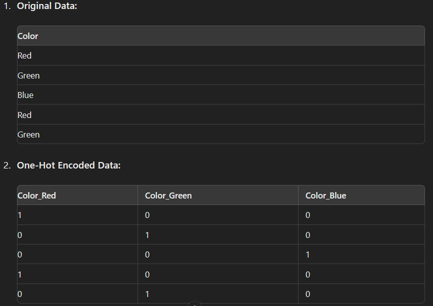
3. Dummy Encoding: Dummy encoding is similar to one-hot encoding, but instead of creating a binary column for each category, it creates n-1 columns for n categories. This avoids redundancy since if all other category columns are 0, the category can be inferred.

4. Binary Encoding: in binary encoding categorical data values are converted into a binary value. It is like one hot encoding however here only log(base 2)n variables are created for n categories. It creates a very less number of variables than one hot encoding.

   

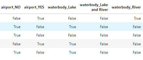
pandas provide inbuilt function to generate all dummy variables

df = pd.get_dummies(df)

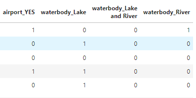
# convert boolean values into integer 1 for true 0 for false
df['airport_YES'] = df['airport_YES'].astype(int)
df['waterbody_Lake'] = df['waterbody_Lake'].astype(int)
df['waterbody_Lake and River'] = df['waterbody_Lake and River'].astype(int)
df['waterbody_River'] = df['waterbody_River'].astype(int)

#airport_YES is sufficient, delete airport_NO
del df['airport_NO']

#the simplest way to do all this
df = pd.get_dummies(df, drop_first=True).astype(int)

6. Correlation Analysis

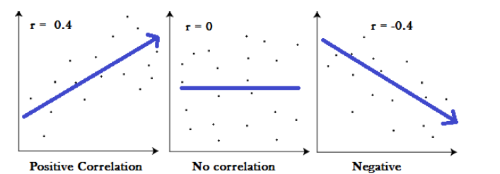
Correlation is a statistical measure that indicates the extent to which two or more variables fluctuate together. A positive correlation indicates the extent to which those variables increase or decrease in parallel; a negative correlation indicates the extent to which one variable increases as the other decreases.

Correlation simply means How two variables are related.

6.1 Correlation Coefficient

• A correlation coefficient is a way to put a value to the relationship.

• Correlation coefficients have a value of between -1 and 1.

• A “0” means there is no relationship between the variables at all,

While -1 or 1 means that there is a perfect negative or positive correlation

6.2 Correlation Matrix

• A correlation matrix is a table showing correlation coefficients between variables.

• Each cell in the table shows the correlation between two variables.

• A correlation matrix is used as a way to summarize data, as an input into a more advanced analysis, and as a diagnostic for advanced analyses.

Note: If two variables have high correlation it means they are linear and dependent variable (y) is in same proportion with both of them, to avoid multicollinearity in modeling we remove one variable based on which has less business sense.

What is Multicollinearity?

• Multicollinearity exists whenever two or more of the predictors in a regression model are moderately or highly correlated.

• Multicollinearity results in a change in the signs as well as in the magnitudes of the partial regression coefficients from one sample to another sample.

Remove highly correlated independent variables by looking at the correlation matrix and VIF

#plot correlation matrix 
df.corr()

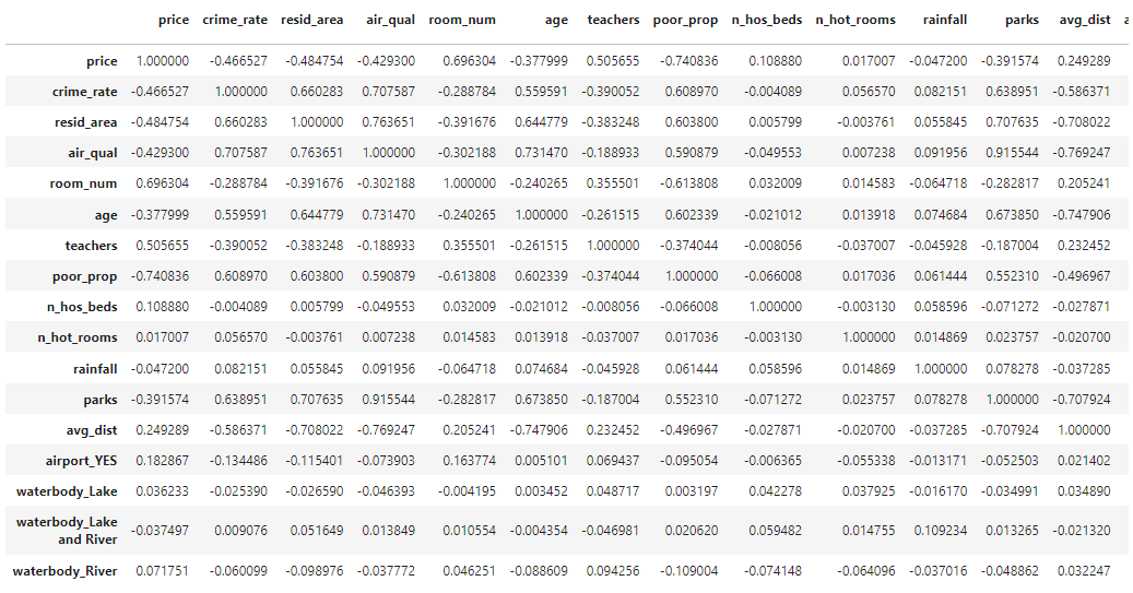
• "parks" and "air_qual" has higher correlation i.e. 0.915544.

• correlation between "price" and "parks" is -0.3915. and that between "price" and "air_qual" is -0.4293.

• price is more dependent on "air_quality", hence we remove parks.

    del df['parks']
  

Conclusion

In this blog, we explored the key steps in data preprocessing for machine learning, including understanding your data, handling outliers, managing missing values, and performing transformations. We repeatedly perform these steps till we get perfect data. These steps are crucial for preparing raw data, ensuring it is clean and ready for modeling, which ultimately enhances the performance of machine learning algorithms.

In next blog, we’ll dive into Linear Regression, a fundamental algorithm in machine learning used for predicting outcomes based on input variables. We’ll cover its core concepts, the underlying math, and how to implement it in Python. This blog will help you understand and apply Linear Regression in practical scenarios.

Stay Tunned, Happy Learning!