Building a Deep Learning Model for Brain Tumor Detection: A Step-by-Step Guide
 Gaurav Bhatnagar
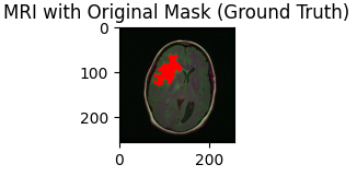
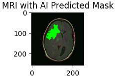
Final Output:


In recent years, deep learning has revolutionized the field of medical imaging, offering unprecedented accuracy in diagnosing complex conditions. Among these, brain tumor detection from MRI scans is a critical application where early and accurate diagnosis can significantly impact patient outcomes. In this blog post, we'll walk through the process of building a deep learning model for brain tumor detection using Python, TensorFlow, and Keras. We will develop 2 separate models to make our predictions. The first model will predict if a brain MRI has a tumor, which will be a binary output of 0 or 1, with 1 indicating positive case. If an MRI does have a tumor, as determined by the first model, then it will be sent to a second deep learning model that will actually make a segmentation mask to display where the tumor is on the given MRI.
Step 1: Setting Up Your Environment
Before diving into the code, it's essential to set up a suitable environment for development. This project is designed to be run on Google Colab, a cloud-based platform that offers free access to GPUs, making it ideal for training deep learning models.
First, we need to import the necessary libraries:
import pandas as pd
import numpy as np
import seaborn as sns
import matplotlib.pyplot as plt
import cv2
import tensorflow as tf
from tensorflow.keras import layers, models, callbacks
from sklearn.preprocessing import StandardScaler, normalize
These libraries provide the tools for data handling, image processing, and model development.
Step 2: Understand the Dataset
Our dataset consists of brain MRI images with their corresponding segmentation masks, which highlight the regions affected by tumors. The masks serve as ground truth for training our model, guiding it to learn the difference between healthy tissues and tumor-affected regions.
brain_df = pd.read_csv('data_mask.csv')
brain_df.info()
brain_df.head()
The data_msk.csv file contains the filepaths to the MRI images and their masks. Understanding the structure of thais dataset is crucial for the next steps, where we'll preprocess the image and feed them into the model.
Step 3: Preprocessing the Data
Medical Imaging requires careful preprocessing of the data to ensure that the model can learn effectively. This includes resizing the images to a consistent shape, normalizing pixel values, and applying data augmentation techniques to improve generalization.
image = cv2.imread(brain_df['image_path'][0])
image = cv2.resize(image, (224, 224))
image = image / 255.0
Here, we use the OpenCV library to read, resize and then normalize the images to have pixel values between 0 and 1. Normalization is particularly important for deep learning models as it stabilizes and speeds up the training process.
Step 4: Building the First Model
Now it's time to build our model. We will leverage transfer learning, a technique where a pre-trained model is fine-tuned on a dataset that is has never seen before. For this model, we will use the ResNet50 and Densenet121 architectures, which have been pre-trained on the 'Imagenet' model wights.
base_model = tf.keras.applications.ResNet50(weights='imagenet', include_top=False, input_shape=(224, 224, 3))
model = models.Sequential([
base_model,
layers.GlobalAveragePooling2D(),
layers.Dense(1, activation='sigmoid')
])
The ResNet50 acts as a feature extractor, and we add a few extra layers for our specific task. The final layer uses the 'sigmoid' activation function, which is used for binary classification-tumor vs no tumor.
Step 5: Training the Classifying Model
Training is where the model learns from the data. We use several callbacks to monitor and adjust the training process, ensuring that the model converges to an optimal solution.
early_stopping = callbacks.EarlyStopping(monitor='val_loss', patience=10)
model_checkpoint = callbacks.ModelCheckpoint('best_model.h5', save_best_only=True)
model.compile(optimizer='adam', loss='binary_crossentropy', metrics=['accuracy'])
EarlyStopping callback halts training if the validation loss does not improve, which prevents overfitting. The ModelCheckpoint will save our best best model based on validation performance, allowing us to display the most accurate model.
Step 6: Evaluating the Model
It is crucial to evaluate our model before we make our own segmentation masks for the MRI's.
model.load_weights('best_model.h5')
test_loss, test_acc = model.evaluate(test_data)
print(f"Test Accuracy: {test_acc:.2f}")
This test accuracy will give us a clear indication of the model's performance. Other metrics to look at it would be precision, recall, and F1 score.
Before we go onto making the segmentation masks for the tumors, take a moment to acknowledge what you have done. You have developed a powerful model that can predict of a given brain MRI has a tumor, already making a big contribution to the real-world. Now let's move on and make tumor masks on the MRI's.
Step 7: Building the Segmentation Model
We have made the classification model, its time to tackle the next step. This is where our second model comes into play. We will be using the U-net architecture, a popular choice for medical image segmentation due to to its ability to capture fine details while maintaining contextual information. Our model will take in the MRI image as input and output a mask that highlights the tumor area.
inputs = layers.Input((224, 224, 3))
c1 = layers.Conv2D(16, (3, 3), activation='relu', padding='same')(inputs)
c1 = layers.Conv2D(16, (3, 3), activation='relu', padding='same')(c1)
p1 = layers.MaxPooling2D((2, 2))(c1)
# Downsampling layers...
# Bottleneck layers...
# Upsampling layers...
outputs = layers.Conv2D(1, (1, 1), activation='sigmoid')(u9)

segmentation_model = models.Model(inputs=[inputs], outputs=[outputs])
segmentation_model.compile(optimizer='adam', loss='binary_crossentropy', metrics=['accuracy'])
The full code for the Downsampling, Bottleneck, and Upsampling layers can be found at the bottom of this page
Step 8: training the Segmentation Model
Just like our classification model, the segmentation model requires training. The key difference here is that our training data consists of both the original MRI images and their corresponding segmentation masks, which serve as ground truth.
# use early stopping to exit training if validation loss is not decreasing even after certain epochs (patience)
earlystopping = EarlyStopping(monitor='val_loss', mode='min', verbose=1, patience=20)

# save the best model with least validation loss
checkpointer = ModelCheckpoint(filepath="classifier-resnet-weights.keras", verbose=1, save_best_only=True)
The same EarlyStopping and CheckPointer techniques are used.
Step 9: Evaluating the model
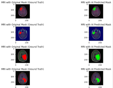
Finally, the moment you have been waiting for. Time to see if our model creates our brain tumor masks. We will test it on some random MRI's from the testing set:

These results are truly amazing as you can see how our AI mask is almost matching the actual tumor location.
Conclusion
Developing a project like this one is challenging yet rewarding task. By leveraging transfer learning and carefully preprocessing the data, we can create these 2 models that can aid in early diagnosis of a brain tumor, potentially saving lives. This project is just a single step into the world of AI in healthcare and how it can be used to solve medical challenges.
Future Work
This project can be taken to the next level by becoming a real-world application. Having it as a software or a mobile app will make brain tumor detection accessible to healthcare providers and patients alike.
Call to Action
If you're interested in applying deep learning to healthcare or want to build similar models, start experimenting with datasets like these and see the impact AI can have. Don’t forget to share your findings and contribute to this exciting field!
Subscribe to my newsletter
Read articles from Gaurav Bhatnagar directly inside your inbox. Subscribe to the newsletter, and don't miss out.
Written by
