Printed Circuit Boards (PCBs) are essential components in modern electronics, providing the foundational structure for electronic circuits. With the increasing complexity of electronic devices, ensuring the quality and reliability of PCBs has become more critical than ever. Defects in PCBs can lead to failures in devices, resulting in costly repairs, product recalls, and damage to brand reputation. To mitigate these risks, automating the detection and identification of PCB defects using advanced machine learning techniques, such as YOLOv5, can be a game-changer.

In this comprehensive guide, we will walk through the entire process of detecting and identifying defects in PCBs using the YOLOv5 model. This process includes data collection, annotation, model training, and evaluation, all executed within a Python and Jupyter Notebook environment.

Step 1: Data Collection and Preparation

The foundation of any machine learning project is data. In our case, we need a dataset that includes images of PCBs with various defects. For this project, we sourced our data from Kaggle, a popular platform for datasets related to machine learning and data science.

The dataset we used includes images with six types of PCB defects: Missing Hole, Mouse Bite, Open Circuit, Short Circuit, Spur, and Spurious Copper. Once the dataset is downloaded, the first step is to extract it and organize the files for further processing.

import zipfile
import os
# Extract the dataset from the zip file
with zipfile.ZipFile('pcb_defects.zip', 'r') as zip_ref:
    zip_ref.extractall('pcb_defects')
# Remove unnecessary files that are not needed for the training process
os.remove('pcb_defects/rotation')
os.remove('pcb_defects/python_file.py')

After extraction, we inspect the contents of the dataset to ensure it contains the necessary images and annotations. The dataset is typically structured with images in one folder and corresponding annotation files in another. For YOLOv5, these annotations must be in a specific format, which leads us to our next step.

Step 2: Data Annotation and Preprocessing

YOLOv5, like other object detection models, requires annotations in a particular format. Each image in the dataset must have an associated text file that contains the bounding box coordinates and class labels for each defect present in the image. Unfortunately, the annotations provided with our dataset were in XML format, which is not directly compatible with YOLOv5. Therefore, we need to convert these XML files to the required text format.

To accomplish this, we use a Python package that automates the conversion of XML annotations to YOLO-compatible text files. This package can be found on GitHub, and the process involves cloning the repository and running the conversion script.

# Clone the repository for converting XML annotations to text format
!git clone https://github.com/user/xml_to_txt.git

Copy all the folders in the Annotation folder to the xml folder in XmlToTxt repo,then run the below comments.

# Install the necessary dependencies from the requirements file
!pip install -r xml_to_txt/requirements.txt# Import the conversion module and run the conversion process
import osos.chdir("XmlToTxt")!python xmltotxt.py -c classes.txt -xml xml -out out

Once the conversion is complete, we verify that each image now has a corresponding text file with annotations in the correct format and are precent in then ‘out’ folder.

Copy all these txt files to the image folder which have the images for training.

Step 3: Split the data for training and testing

For the yolo training the dataset folder has to be in the below particular format.

Dataset/
│
├── images/
│   ├── train/
│   └── val/
│
└── labels/
    ├── train/
    └── val/

For this purpose we have run the below code, which moves the images and labels to this particular yolo directory structure

import os
from random import choice
import shutil
def to_v5_directories(images_train_path,images_val_path,labels_train_path,labels_val_path, dataset_source):
    imgs =[]
    xmls =[]
    trainPath = images_train_path
    valPath =  images_val_path
    crsPath = dataset_source
    train_ratio = 0.8
    val_ratio = 0.2
    totalImgCount = len(os.listdir(crsPath))/2
    for (dirname, dirs, files) in os.walk(crsPath):
        for filename in files:
            if filename.endswith('.txt'):
                xmls.append(filename)
            else:
                imgs.append(filename)
    countForTrain = int(len(imgs)*train_ratio)
    countForVal = int(len(imgs)*val_ratio)
    trainimagePath = images_train_path
    trainlabelPath = labels_train_path
    valimagePath = images_val_path
    vallabelPath = labels_val_path
    for x in range(countForTrain):
        fileJpg = choice(imgs)
        fileXml = fileJpg[:-4] +'.txt'
        shutil.copy(os.path.join(crsPath, fileJpg), os.path.join(trainimagePath, fileJpg))
        shutil.copy(os.path.join(crsPath, fileXml), os.path.join(trainlabelPath, fileXml))
        imgs.remove(fileJpg)
        xmls.remove(fileXml)
    for x in range(countForVal):
        fileJpg = choice(imgs) 
        fileXml = fileJpg[:-4] +'.txt' 
        shutil.copy(os.path.join(crsPath, fileJpg), os.path.join(valimagePath, fileJpg))
        shutil.copy(os.path.join(crsPath, fileXml), os.path.join(vallabelPath, fileXml))
        imgs.remove(fileJpg)
        xmls.remove(fileXml)
    print("Training images are : ",countForTrain)
    print("Validation images are : ",countForVal)
#     shutil.move(crsPath, valPath)

Then run this to split the images and labels for training and validation.

to_v5_directories("PCB_DATASET/dataset/images/train","PCB_DATASET/dataset/images/val","PCB_DATASET/dataset/labels/train","PCB_DATASET/dataset/labels/val", "PCB_DATASET/Annotations/{each_image_gropu}")

Step 4: Setting Up and Training the YOLOv5 Model

With our dataset prepared and annotations in place, we move on to the training phase. YOLOv5 is a state-of-the-art object detection model known for its speed and accuracy. To train the model, we need to set up the environment, load the dataset, and configure the training parameters.

We opted to use Google Colab for training, leveraging its GPU support to accelerate the process. The first step is to upload the dataset to Google Drive and mount the drive in the Colab environment.

Then zip the dataset folder and upload to your gogle drive.p

from google.colab import drive
drive.mount('/content/drive')

# Unzip and prepare the dataset within the Google Colab environment
!unzip -q "/content/drive/My Drive/PCB_DATASET.zip" -d /content/

Next, we clone the YOLOv5 repository from GitHub and install the necessary dependencies. This repository includes the pre-trained weights, configuration files, and training scripts needed to train the model on our PCB dataset.

!git clone https://github.com/ultralytics/yolov5.git

# Change the directory to the cloned YOLOv5 repository
%cd yolov5# Install the required dependencies for YOLOv5
!pip install -r requirements.txt

Configuring the Dataset

Before training, we need to configure the dataset by creating a dataset.yaml file. This file defines the paths to the training and validation datasets, the number of classes, and their names. This configuration ensures that YOLOv5 understands the structure of our data.

# Content of dataset.yaml
train: /content/PCB_DATASET/dataset/images/train
val: /content/PCB_DATASET/dataset/images/val
# Number of classes in the dataset
nc: 6
# Class names
names: ['Missing_Hole', 'Mouse_Bite', 'Open_Circuit', 'Short_Circuit', 'Spur', 'Spurious_Copper']

This YAML file is then uploaded to the YOLOv5 directory in Colab, and we are ready to start training the model.

Training the YOLOv5 Model

Training the YOLOv5 model involves specifying several parameters, such as the image size, batch size, number of epochs, and the type of YOLOv5 model to use. YOLOv5 offers several model sizes, ranging from the small and fast YOLOv5n to the larger and more accurate YOLOv5x.

# Training the YOLOv5 model
!python train.py --img 640 --batch 16 --epochs 300 --data dataset.yaml --weights yolov5s.pt --project pcb_defects_run1

In this command:

--img 640 specifies the input image size.
--batch 16 sets the batch size for training.
--epochs 300 sets the number of training iterations. More epochs can lead to better accuracy but also require more time.
--data dataset.yaml points to our dataset configuration file.
--weights yolov5s.pt specifies the pre-trained YOLOv5 model weights to be used.
--pcb_defect_run1 names the output directory where the training results will be stored.

Training begins, and the model iteratively improves as it learns to detect and classify PCB defects.

Step 5: Evaluating the Model

Once training is complete, evaluating the model’s performance is crucial. YOLOv5 provides several tools to assess the model, including precision-recall curves, confusion matrices, and other metrics. These evaluations help us understand how well the model is detecting and classifying defects.

With the number of epochs as 300, the model’s accuracy is shown as 93%.

import matplotlib.pyplot as plt
from IPython.display import Image

# Display the confusion matrix for the trained model
Image('runs/train/pcb_defects/confusion_matrix.png')# Display the precision-recall curve
Image('runs/train/pcb_defects/PR_curve.png')

The precision-recall curve and confusion matrix are particularly useful for understanding how well the model differentiates between the various defect types. These tools allowed us to fine-tune the model for better performance.

Step 6: Validating and Predicting

With a well-trained model, the final step is to validate it using a separate validation dataset and make predictions on new images. This step ensures that the model generalizes well to unseen data and can accurately detect and classify PCB defects in real-world scenarios.

# Run the model on validation images and display the results
!python val.py --weights runs/train/pcb_defects/weights/best.pt --data dataset.yaml

# Visualize the predicted results on a sample image
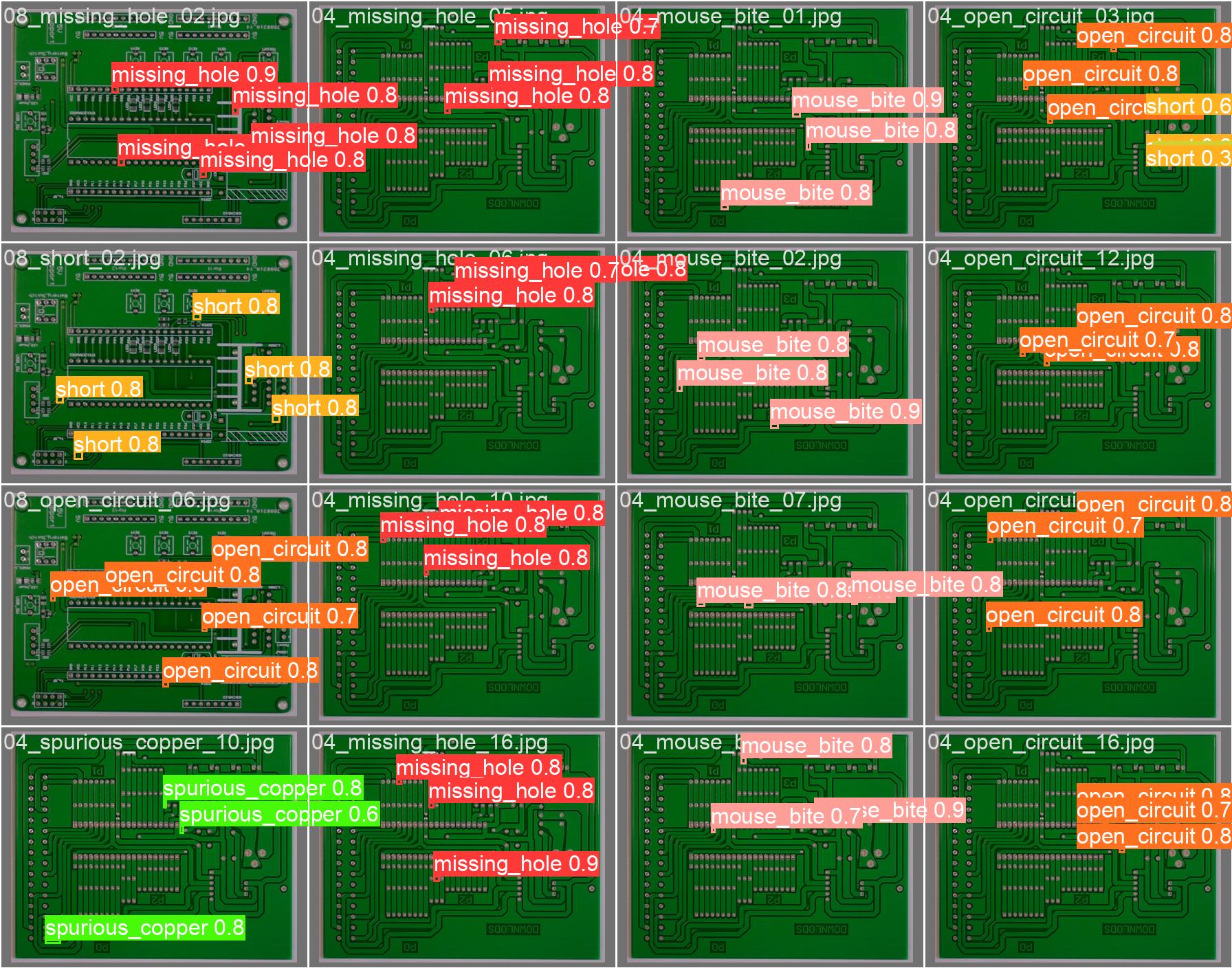
Image('runs/val/pcb_defects/predictions.jpg')

The model’s predictions were significantly improved after increasing the number of training epochs. The model is now capable of accurately detecting defects in PCBs, making it a valuable tool for automating quality control in electronics manufacturing.

Step 7: Analysing the Confusion Matrix and Precision-Recall Curve

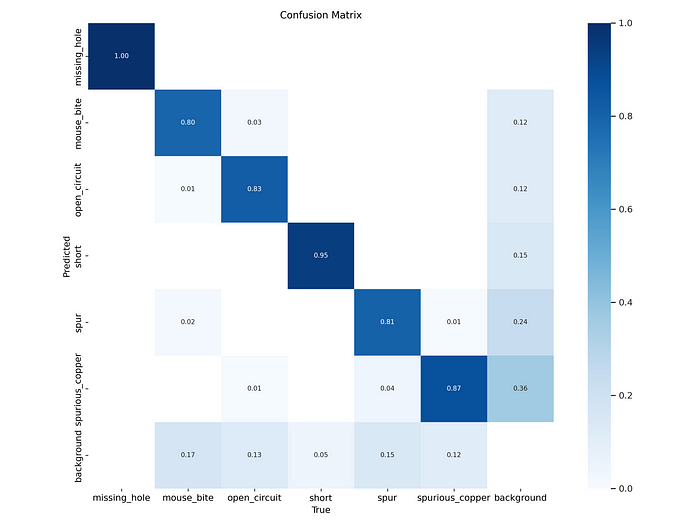
The confusion matrix provides a detailed breakdown of the model’s performance across different defect categories. Each row represents the predicted class, while each column represents the actual class. Here’s a breakdown of what the confusion matrix tells us about the model’s performance:

Missing Hole: The model has a perfect prediction accuracy for the ‘Missing Hole’ class, as indicated by a value of 1.00 in the corresponding cell. This means every ‘Missing Hole’ defect was correctly identified.
Mouse Bite: The model achieved an accuracy of 0.80 for the ‘Mouse Bite’ class, with a slight misclassification of 0.03 as ‘Spurious Copper’. This indicates that the model generally performs well on this class but has room for improvement in distinguishing it from similar defects.
Open Circuit: The model correctly identified ‘Open Circuit’ defects with an accuracy of 0.83. However, 12% of these defects were misclassified as ‘Spurious Copper’, which suggests that these two classes might have overlapping features that confuse the model.
Short Circuit: The model showed high accuracy (0.95) in detecting ‘Short Circuit’ defects, with minimal misclassification, indicating that this class is well-represented in the training data or that the features are distinct.
Spur: The model struggled with the ‘Spur’ class, showing a lower accuracy of 0.81 and a significant confusion with ‘Spurious Copper’ (0.24). This suggests that the features of ‘Spur’ defects are often mistaken for those of ‘Spurious Copper’.
Spurious Copper: The accuracy for ‘Spurious Copper’ is 0.87, but there is considerable misclassification with the background (0.36), indicating that the model sometimes confuses this defect with non-defect areas.

Precision-Recall Curve Analysis

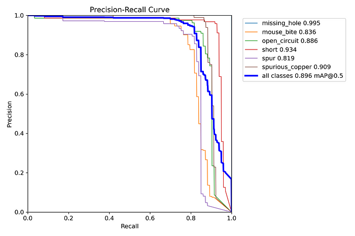
The Precision-Recall (PR) curve further provides insights into the model’s ability to handle the imbalance between the positive class (defects) and the negative class (background or no defect).

Overall Performance: The mean Average Precision (mAP@0.5) for all classes is 0.896, which is a strong indicator of the model’s overall performance.
Class-Specific Performance:
Missing Hole: Exhibits near-perfect precision and recall (0.995), affirming its ease of detection by the model.
Mouse Bite: Has a lower precision (0.836), which suggests that while the model is generally accurate, there are a few instances where the model incorrectly predicts this class.
Open Circuit: The precision is 0.886, showing that the model is fairly good at detecting this class but still misclassifies some defects.
Short Circuit: With a precision of 0.934, this class is well-detected, aligning with the confusion matrix results.
Spur: This class has the lowest precision at 0.819, reflecting the confusion noted in the confusion matrix. This might require further model refinement or more data.
Spurious Copper: With a precision of 0.909, the model performs well on this class, but there is still some misclassification that lowers the score.

8. Conclusion

The confusion matrix and precision-recall curve together paint a detailed picture of the model’s strengths and weaknesses in detecting PCB defects. The model excels in detecting ‘Missing Hole’ and ‘Short Circuit’ defects but shows some confusion between similar defect types like ‘Spur’ and ‘Spurious Copper’.

Improving the model might involve increasing the number of epochs, augmenting the dataset, or fine-tuning the model parameters to better distinguish between the more similar defect types. Despite some areas for improvement, the overall performance of the model is strong, making it a valuable tool for automated PCB defect detection.

Comprehensive Guide to Detecting and Identifying Defects in PCBs Using YOLOv5