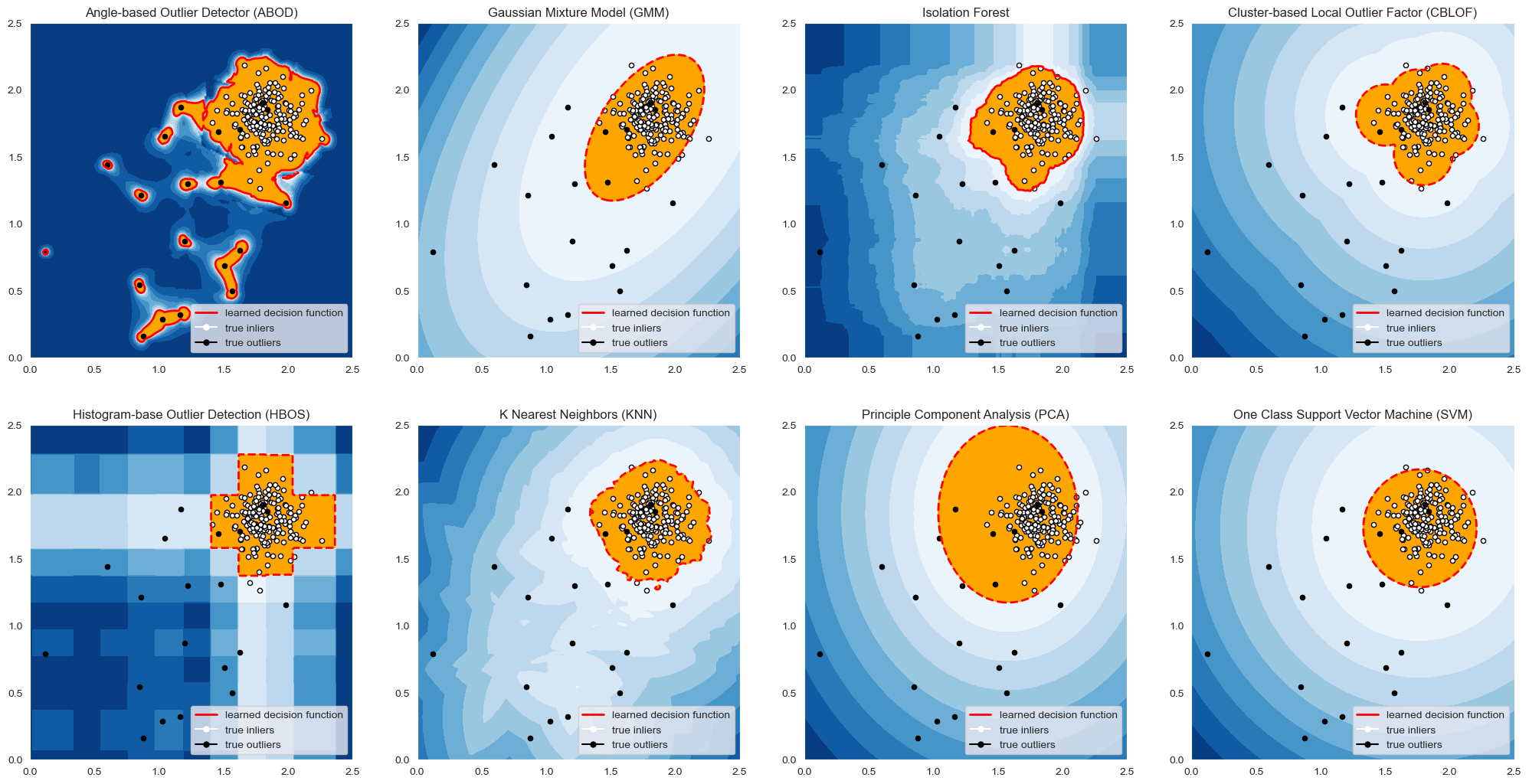
Table of Contents

1. Introduction

2. Key Areas of Anomaly Detection in Building Management

• 2.1 Proactive Maintenance

• 2.2 Energy Efficiency

• 2.3 Occupant Comfort

3. Understanding the Algorithms

• 3.1 Angle-Based Outlier Detector (ABOD)

• 3.2 Gaussian Mixture Model (GMM)

• 3.3 Isolation Forest

• 3.4 Cluster-Based Local Outlier Factor (CBLOF)

• 3.5 Histogram-Based Outlier Detection (HBOS)

• 3.6 K-Nearest Neighbors (KNN)

• 3.7 Principal Component Analysis (PCA)

• 3.8 Support Vector Machine (SVM)

4. Applying the Algorithms to Building Data

• 4.1 Loading and Preprocessing the Data

• 4.2 Unsupervised Anomaly Detection

• 4.3 Supervised Anomaly Detection

5. Resulting Plots

6. Conclusion and Future Work

7. References

1. Introduction

Buildings today are more than just physical structures; they are complex ecosystems embedded with sensors that continuously monitor various parameters such as temperature, humidity, energy consumption, and occupancy levels. This wealth of data presents an opportunity to not only manage building operations more efficiently but also to preemptively address potential issues through anomaly detection.

Anomalies in building data could indicate equipment failures, energy inefficiencies, or deviations in occupancy patterns that might signal security concerns. By employing machine learning techniques to detect these anomalies, building managers can transform their facilities into smart environments capable of proactive maintenance, optimized energy consumption, and enhanced occupant comfort.

In this comprehensive guide, we will explore a variety of machine learning algorithms for anomaly detection, applying both unsupervised and supervised methods to real-world building data. We will delve into the strengths and weaknesses of each approach, supported by detailed code snippets and visualizations.

2. Key Areas of Anomaly Detection in Building Management

Anomaly detection in building data is crucial for several reasons:

2.1 Proactive Maintenance

• Identifying anomalies in equipment performance allows for early intervention, reducing the likelihood of major failures. This not only minimizes downtime but also extends the life of critical systems, ultimately saving costs on repairs and replacements.

2.2 Energy Efficiency

• Buildings consume a significant amount of energy, and even minor inefficiencies can lead to substantial waste. Anomaly detection can pinpoint irregularities in energy usage, enabling targeted interventions to reduce consumption, lower operational costs, and support sustainability initiatives.

2.3 Occupant Comfort

• Comfort is paramount in residential and commercial spaces. Anomalies in environmental data (e.g., temperature, air quality) can lead to uncomfortable conditions for occupants. By detecting these issues early, building managers can take corrective action to maintain a pleasant and safe environment.

3. Understanding the Algorithms

Various machine learning algorithms are employed for anomaly detection, each with its unique strengths and application scenarios. Here’s a deeper dive into some of the most effective methods:

3.1 Angle-Based Outlier Detector (ABOD)

• Concept: ABOD evaluates the angle between pairs of data points with respect to the origin. Points with smaller angles compared to the majority are considered outliers.

• Application: Useful in high-dimensional data where traditional distance-based methods may struggle.

Code:

from pyod.models.abod import ABOD
abod = ABOD()
abod.fit(preprocessed_data[['CO2', 'electricity']])
preprocessed_data['abod_anomaly'] = abod.labels_
# Plotting
plt.figure(figsize=(10, 6))
plt.scatter(preprocessed_data['CO2'], preprocessed_data['electricity'], c=preprocessed_data['abod_anomaly'], cmap='coolwarm')
plt.title('ABOD Anomaly Detection')
plt.xlabel('CO2 Levels')
plt.ylabel('Electricity Consumption')
plt.show()

3.2 Gaussian Mixture Model (GMM)

• Concept: GMM assumes that the data is a mixture of several Gaussian distributions. It estimates the parameters (mean and covariance) of these distributions and assigns a likelihood to each data point. Points with low likelihood are flagged as anomalies.

• Application: Effective when the data naturally clusters around multiple centers (e.g., different operating states of a building system).

Code:

from sklearn.mixture import GaussianMixture
gmm = GaussianMixture(n_components=2)
gmm.fit(preprocessed_data[['CO2', 'electricity']])
scores = gmm.score_samples(preprocessed_data[['CO2', 'electricity']])
preprocessed_data['gmm_anomaly'] = (scores < threshold).astype(int)
# Plotting
plt.figure(figsize=(10, 6))
plt.scatter(preprocessed_data['CO2'], preprocessed_data['electricity'], c=preprocessed_data['gmm_anomaly'], cmap='coolwarm')
plt.title('GMM Anomaly Detection')
plt.xlabel('CO2 Levels')
plt.ylabel('Electricity Consumption')
plt.show()

3.3 Isolation Forest

• Concept: Isolation Forest isolates observations by randomly selecting a feature and then randomly selecting a split value between the maximum and minimum values of the selected feature. The algorithm is based on the premise that anomalies are few and different, making them easier to isolate.

• Application: Widely used for its efficiency and scalability, especially in large datasets.

Example Code:

from sklearn.ensemble import IsolationForest
isolation_forest = IsolationForest(contamination=0.01)
preprocessed_data['iforest_anomaly'] = isolation_forest.fit_predict(preprocessed_data[['CO2', 'electricity']])
# Identifying anomalies
anomalies = preprocessed_data[preprocessed_data['iforest_anomaly'] == -1]
# Plotting
plt.figure(figsize=(10, 6))
plt.plot(preprocessed_data['timestamp'], preprocessed_data['CO2'], label='CO2 Levels')
plt.scatter(anomalies['timestamp'], anomalies['CO2'], color='red', label='Anomaly', marker='x')
plt.title('CO2 Levels with Anomalies Detected by Isolation Forest')
plt.xlabel('Timestamp')
plt.ylabel('CO2 Levels')
plt.legend()
plt.show()

3.4 Cluster-Based Local Outlier Factor (CBLOF)

• Concept: CBLOF calculates the local outlier factor for each data point by comparing its distance to its closest cluster centroid. Points that deviate significantly from their cluster are considered outliers.

• Application: Suitable for data where natural clusters exist, such as different operational modes of HVAC systems.

Code:

from pyod.models.cblof import CBLOF
cblof = CBLOF()
cblof.fit(preprocessed_data[['CO2', 'electricity']])
preprocessed_data['cblof_anomaly'] = cblof.labels_
# Plotting
plt.figure(figsize=(10, 6))
plt.scatter(preprocessed_data['CO2'], preprocessed_data['electricity'], c=preprocessed_data['cblof_anomaly'], cmap='coolwarm')
plt.title('CBLOF Anomaly Detection')
plt.xlabel('CO2 Levels')
plt.ylabel('Electricity Consumption')
plt.show()

3.5 Histogram-Based Outlier Detection (HBOS)

• Concept: HBOS is a fast, unsupervised method that segments the data into bins (histograms) and assigns an anomaly score based on the density of each bin. Outliers are detected in regions with low density.

• Application: Effective in large datasets where speed is critical, such as real-time monitoring systems.

Code:

from pyod.models.hbos import HBOS
hbos = HBOS()
hbos.fit(preprocessed_data[['CO2', 'electricity']])
preprocessed_data['hbos_anomaly'] = hbos.labels_
# Plotting
plt.figure(figsize=(10, 6))
plt.scatter(preprocessed_data['CO2'], preprocessed_data['electricity'], c=preprocessed_data['hbos_anomaly'], cmap='coolwarm')
plt.title('HBOS Anomaly Detection')
plt.xlabel('CO2 Levels')
plt.ylabel('Electricity Consumption')
plt.show()

3.6 K-Nearest Neighbors (KNN)

• Concept: KNN detects anomalies by comparing each data point to its nearest neighbors. If a point is significantly different from its neighbors, it is considered an anomaly.

• Application: KNN is simple yet powerful, making it a popular choice for various anomaly detection tasks.

Code:

from pyod.models.knn import KNN
knn = KNN()
knn.fit(preprocessed_data[['CO2', 'electricity']])
preprocessed_data['knn_anomaly'] = knn.labels_
# Plotting
plt.figure(figsize=(10, 6))
plt.scatter(preprocessed_data['CO2'], preprocessed_data['electricity'], c=preprocessed_data['knn_anomaly'], cmap='coolwarm')
plt.title('KNN Anomaly Detection')
plt.xlabel('CO2 Levels')
plt.ylabel('Electricity Consumption')
plt.show()

3.7 Principal Component Analysis (PCA)

• Concept: PCA reduces the dimensionality of the data by transforming it into a set of orthogonal components. Anomalies are detected as points that do not align with the main axes of the data.

• Application: Ideal for high-dimensional data where traditional methods may be less effective.

Code:

from sklearn.decomposition import PCA
pca = PCA(n_components=2)
transformed_data = pca.fit_transform(preprocessed_data[['CO2', 'electricity']])
preprocessed_data['pca_anomaly'] = (np.abs(transformed_data) > threshold).any(axis=1).astype(int)
# Plotting
plt.figure(figsize=(10, 6))
plt.scatter(transformed_data[:, 0], transformed_data[:, 1], c=preprocessed_data['pca_anomaly'], cmap='coolwarm')
plt.title('PCA Anomaly Detection')
plt.xlabel('PCA Component 1')
plt.ylabel('PCA Component 2')
plt.show()

3.8 Support Vector Machine (SVM)

• Concept: SVM constructs a hyperplane in a high-dimensional space that separates normal data points from anomalies. Data points that lie on the wrong side of the hyperplane are considered outliers.

• Application: SVM is a versatile and effective method, particularly in datasets with complex, non-linear boundaries.

Example Code:

from sklearn.svm import OneClassSVM
svm = OneClassSVM(gamma='auto')
svm.fit(preprocessed_data[['CO2', 'electricity']])
preprocessed_data['svm_anomaly'] = svm.predict(preprocessed_data[['CO2', 'electricity']])
# Plotting
plt.figure(figsize=(10, 6))
plt.scatter(preprocessed_data['CO2'], preprocessed_data['electricity'], c=preprocessed_data['svm_anomaly'], cmap='coolwarm')
plt.title('SVM Anomaly Detection')
plt.xlabel('CO2 Levels')
plt.ylabel('Electricity Consumption')
plt.show()

4. Applying the Algorithms to Building Data

We applied these algorithms to a real-world dataset from the Lawrence Berkeley National Laboratory, focusing on indoor CO2 levels and miscellaneous electrical consumption. Here’s a detailed analysis of how each algorithm performed:

4.1 Loading and Preprocessing the Data

Before diving into anomaly detection, it’s crucial to preprocess the data. This step includes cleaning the data, handling missing values, and scaling features to ensure that the algorithms perform optimally.

import pandas as pd
import numpy as np
from utils import preprocess_data
# Load the dataset
data = pd.read_csv('building_data.csv')
# Preprocess the data
preprocessed_data = preprocess_data(data)
# Scaling the data
from sklearn.preprocessing import StandardScaler
scaler = StandardScaler()
preprocessed_data[['CO2', 'electricity']] = scaler.fit_transform(preprocessed_data[['CO2', 'electricity']])

4.2 Unsupervised Anomaly Detection

We began with unsupervised methods, which do not require labeled data. These methods are particularly useful when we do not have a pre-defined notion of what constitutes an anomaly.

Example: Isolation Forest

Isolation Forest is a robust and scalable method for detecting anomalies. It works by isolating observations by randomly selecting a feature and then randomly selecting a split value between the maximum and minimum values of the selected feature.

from sklearn.ensemble import IsolationForest
# Initialize and fit the model
isolation_forest = IsolationForest(contamination=0.01)
preprocessed_data['iforest_anomaly'] = isolation_forest.fit_predict(preprocessed_data[['CO2', 'electricity']])
# Identifying anomalies
anomalies = preprocessed_data[preprocessed_data['iforest_anomaly'] == -1]
# Plotting
plt.figure(figsize=(10, 6))
plt.plot(preprocessed_data['timestamp'], preprocessed_data['CO2'], label='CO2 Levels')
plt.scatter(anomalies['timestamp'], anomalies['CO2'], color='red', label='Anomaly', marker='x')
plt.title('CO2 Levels with Anomalies Detected by Isolation Forest')
plt.xlabel('Timestamp')
plt.ylabel('CO2 Levels')
plt.legend()
plt.show()

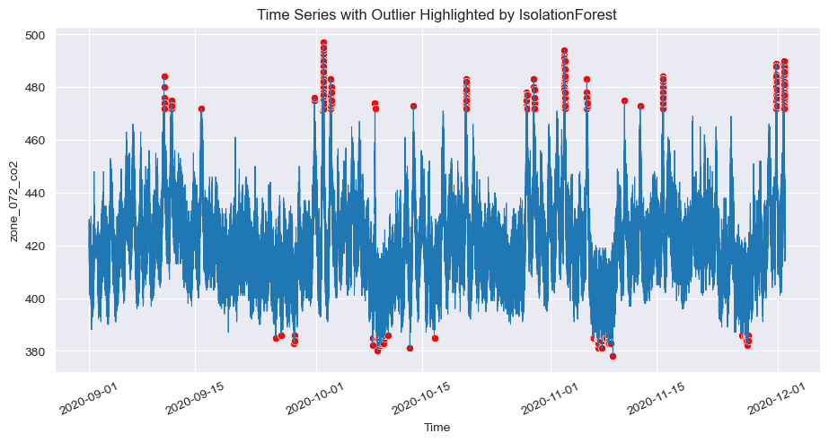
In this example, Isolation Forest effectively identified peaks in CO2 levels that deviate from the norm, flagging them as anomalies. This is crucial for early detection of potential ventilation issues in buildings.

4.3 Supervised Anomaly Detection

Next, we employed supervised methods, which require labeled data. These methods are powerful when historical data with known anomalies is available, allowing the model to learn the patterns associated with normal and anomalous behavior.

Example: Long Short-Term Memory (LSTM)

LSTM networks are a type of recurrent neural network (RNN) well-suited for time series forecasting and anomaly detection. They are capable of learning long-term dependencies in sequential data, making them ideal for detecting anomalies in time series data like CO2 levels or energy consumption.

from tensorflow.keras.models import Sequential
from tensorflow.keras.layers import LSTM, Dense

# Prepare the data for LSTM
X_train, y_train = prepare_lstm_data(preprocessed_data['CO2'])
# Build the LSTM model
model = Sequential()
model.add(LSTM(units=50, return_sequences=True, input_shape=(X_train.shape[1], 1)))
model.add(LSTM(units=50))
model.add(Dense(1))
# Compile and fit the model
model.compile(optimizer='adam', loss='mean_squared_error')
model.fit(X_train, y_train, epochs=20, batch_size=32)
# Predict anomalies
predictions = model.predict(X_train)
anomalies = np.where(np.abs(predictions - y_train) > threshold)[0]
# Plotting
plt.figure(figsize=(10, 6))
plt.plot(y_train, label='True CO2 Levels')
plt.plot(predictions, label='Predicted CO2 Levels')
plt.scatter(anomalies, y_train[anomalies], color='red', label='Anomaly', marker='x')
plt.title('CO2 Levels with Anomalies Detected by LSTM')
plt.xlabel('Time Step')
plt.ylabel('CO2 Levels')
plt.legend()
plt.show()

In this example, the LSTM model predicted CO2 levels based on past data. Significant deviations between predicted and actual values were flagged as anomalies, highlighting periods where the building’s ventilation system might have underperformed.

5. Resulting Plots

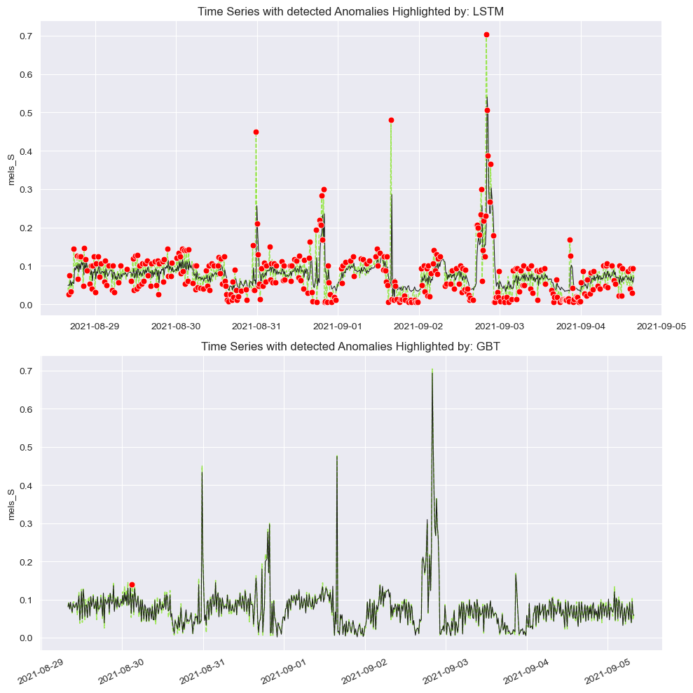
5.1. LSTM and Gradient Boosted Trees (GBT) Anomaly Detection:

• The first plot showcases anomalies detected in a time series by an LSTM (Long Short-Term Memory) model. The LSTM highlights numerous anomalies (marked in red), especially during peaks and fluctuations in the time series, indicating its sensitivity to abrupt changes.

• The second plot uses Gradient Boosted Trees (GBT) for anomaly detection on the same dataset. GBT is more conservative, detecting fewer anomalies compared to LSTM, primarily flagging significant peaks. This comparison highlights the differences in sensitivity between the two models.

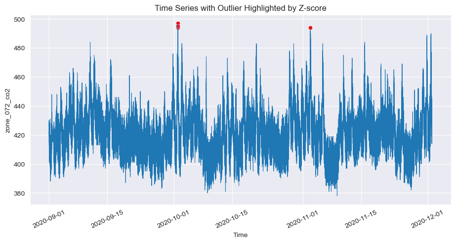
5.2 Z-Score Anomaly Detection:

• The plot shows anomaly detection using the Z-Score method. This method highlights outliers where the data significantly deviates from the mean, as seen in the few points (marked in red) during extreme peaks in the time series. Z-Score is effective at identifying anomalies based on statistical thresholds.

5.3. Isolation Forest Anomaly Detection:

• The plot presents anomalies detected by the Isolation Forest algorithm. This method detects anomalies throughout the time series, including both peaks and troughs, marked in red. Isolation Forest is known for its ability to identify outliers by isolating points that differ significantly from the majority.

5.4. Local Outlier Factor (LOF) Anomaly Detection:

• The fifth plot illustrates anomalies detected by the Local Outlier Factor (LOF). LOF identifies anomalies based on the density of points, detecting areas where points are significantly less dense compared to their neighbors. The red marks indicate anomalies in both high and low regions of the time series.

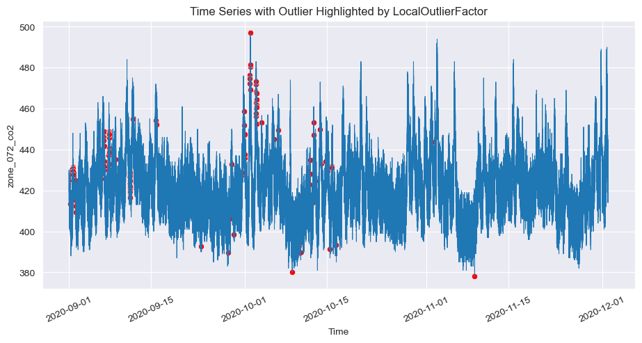
These plots demonstrate how different anomaly detection algorithms highlight outliers in various sections of the time series data, each with its unique sensitivity and approach. The choice of algorithm impacts the type and number of anomalies detected, providing insights into the dataset’s behavior under different analysis techniques.

6. Conclusion and Future Work

This analysis illustrates the importance of selecting the right algorithm for anomaly detection in building data. Each method has its strengths and weaknesses, and the choice of algorithm should be informed by the specific characteristics of the data and the operational goals.

Key Takeaways:

1. Isolation Forest: Effective and scalable, making it suitable for large datasets with complex patterns.

2. LSTM: Powerful for time series data, especially when long-term dependencies are present.

3. ABOD, GMM, CBLOF, HBOS, KNN, PCA, SVM: Each of these methods offers unique advantages depending on the data’s nature and the specific anomalies of interest.

Future Work:

• Threshold Tuning: Adjusting the threshold values for algorithms like LSTM and Isolation Forest could improve the accuracy of anomaly detection.

• Model Ensemble: Combining multiple models might yield more robust results by leveraging the strengths of different approaches.

• Real-Time Monitoring: Implementing these models in a real-time monitoring system could provide continuous insights into building performance, enabling immediate action when anomalies are detected.

By continuously refining these models and algorithms, we can move closer to creating truly intelligent buildings that anticipate and respond to changes, ensuring comfort, safety, and cost-effectiveness.

7. References

1. My Github repo

2. Referred models