EDA is the initial step in data analysis, where we summarize and visualize the main characteristics of a dataset. Descriptive statistics, like mean, median, mode, variance, and standard deviation, help us understand the central tendencies and spread of the data. Through visualizations like histograms, boxplots, and scatter plots, EDA allows us to spot trends, patterns, and potential outliers, setting the stage for deeper analysis.

In today's data-driven world, making informed business decisions is more critical than ever. But with mountains of data at our fingertips, how do we transform raw numbers into meaningful insights? Enter the world of statistical moments—a powerful framework that helps us understand, interpret, and leverage data to its fullest potential.

Whether you're navigating through central tendencies, exploring the depths of data dispersion, or uncovering the hidden patterns of distribution, each moment holds the key to unlocking deeper insights. But it's not just about the numbers; it's about mastering the tools and techniques that turn data into a story—your story.

In this blog, we'll take you on a journey through the four fundamental moments of statistics, breaking down complex concepts into digestible, actionable steps. From measuring the average tendencies of your data to understanding the subtle asymmetries and peaks, we'll equip you with the knowledge to make smarter, data-driven decisions.

FIRST MOMENT BUSINESS DECISION: Measure of Central Tendency

Mean (μ):
- The mean is sensitive to outliers because it factors in every data point. It's best used with symmetrically distributed data without outliers.
- Average : μ = Sum of observations / Total No. of observations [Σ X / N]
- Function: mean()
Median:
- Less sensitive to outliers, making it ideal for skewed distributions.
- Middlemost value of an ordered dataset
- In case of even records, Median is the average of the middle two records
- In Python, use numpy.median() or pandas.Series.median().
Mode:
- Useful for categorical data and identifying the most frequent observation.
- Bimodal Mode: Two records repeated the same number of times
- Multimodal Mode: More than two records repeated the same number of times
- Python's statistics.mode() or scipy.stats.mode() can be used.

SECOND MOMENT BUSINESS DECISION: Measure of Dispersion or Deviation

Variance (σ^2):
- It measures the spread of the data points around the mean.
- Average of squared distances
- σ^2 = Σ (X - μ)^2 / N
- Function: var()
- Use numpy.var() or pandas.Series.var().
Standard Deviation (σ):
- Represents the average distance from the mean.
- Square root of Variance
- σ = √variance
- σ = √Σ [(X-μ)²/N]
- Function: std()
- Use numpy.std() or pandas.Series.std().
Range:
- Maximum value - Minimum value
- Python does not have standard function for range. So, -Function: max() - min()

THIRD MOMENT BUSINESS DECISION: Measure of Asymmetry in distribution

It speaks about the distribution of data
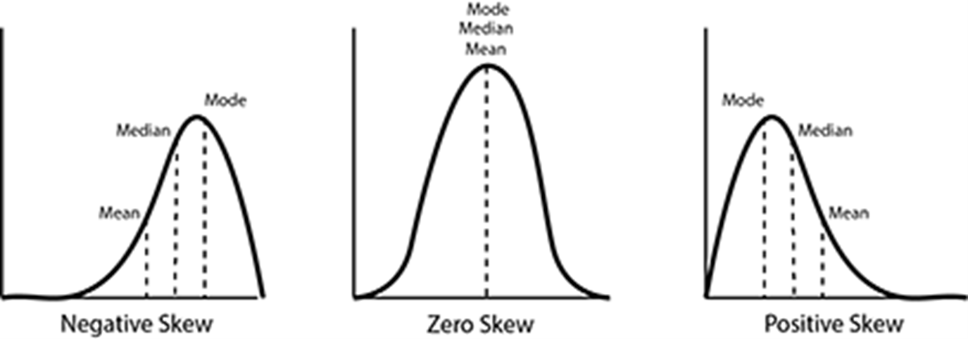
Skewness: Indicates the direction and extent of asymmetry in data.
- Use scipy.stats.skew() for calculation
  - Positive Skewness: Exceptions towards the right
  - Negative Skewness: Exceptions towards the left
  - Skewness = ∑ [(X - μ) / σ]^3
  - If Skew = 0, it’s normal distribution
  - Function: skew()

FOURTH MOMENT BUSINESS DECISION:

Measure of Peakedness in the Distribution
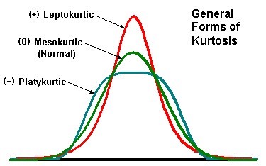
Kurtosis: Measures the "tailedness" of the distribution.
- Use scipy.stats.kurtosis().
  - Positive Kurtosis: Higher peak & long tails
  - Negative Kurtosis: Wider peak & no tails
  - Kurtosis = E[X-μ/σ]⁴-3
  - Bell-shaped curve is considered standard with kurtosis = 3 (Mesokurtic)
  - Function: kurt()
  - Types of Kurtosis:
    - MESOKURTIC - Name of Standard kurtosis curve.(Kurtosis ≈ 0)
    - LEPTOKURTIC - Name of Positive kurtosis curve. (Kurtosis > 0)
    - PLATYKURTIC- Name of Negative kurtosis curve. (Kurtosis < 0)

GRAPHICAL REPRESENTATION

For visualizations, either matplotlib or seaborn package is used. In matplotlib package, pyplot sub package is used for memory optimization.

Boxplot:

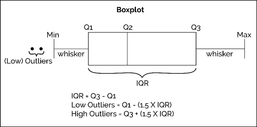
Also called as Box & Whisker plot.
- seaborn.boxplot() or matplotlib.pyplot.boxplot() can be used for creating boxplots.
  - Shows Outliers, uses Q ± 1.5(IQR) to identify limits
    - Where IQR = Q3-Q1
      
      Q1- 25th Percentile
      
      Q2- 50th Percentile/Median
      
      Q3-75th Percentile
  - Function- boxplot() by default boxplot output is vertical. In order to change the direction use parameter called vert.
  - Parameter Vert = True/1, vertical boxplot is obtained.
    
    Vert = False/0, horizontal boxplot is obtained.
    
    By default, vert = True/1.
Barplot:
- Function: bar(X, height)
- Use seaborn.barplot() or matplotlib.pyplot.bar() for bar plots.
- It’s important to note that bar plots are typically used for categorical data.
- For parameters height & X, pass data and index as inputs respectively. Since index is set of sequential numbers, there are 3 syntax's in Python.
  - Syntax's for sequential numbers - [Start, Stop, Step size]
    - Step size value by default is 1.
    - Start value by default is 0.
    - Stop value is n-1.
  - Use range(), np.arange() functions and [Start:Stop:Stepsize]
Histogram:
- Function: hist()
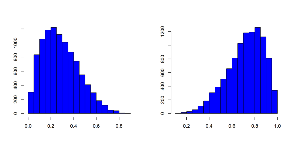
- Use matplotlib.pyplot.hist() or seaborn.histplot().
- Useful for visualizing the distribution of continuous data.
- Data is left or right skewed can be visualized.

DATA CLEANSING/MUNGING/WRANGLING/ORGANIZING

Typecasting:
- Conversion of one data type to another
- pandas.DataFrame.astype() allows you to convert data types.
- Due to dynamic programming nature of Python, data types are assigned to data.
- Function - dtypes gives inferred data types by Python.
- Function: astype() casts pandas object to specified data type.
Handling Duplicates:
- When two or more rows have same records then they are said to be Duplicates.
- pandas.DataFrame.duplicated() and pandas.DataFrame.drop_duplicates() are essential for handling duplicate data.
- Function- duplicated() identifies whether a row is duplicate or not. So, the output is Boolean series (True/False).
  - Parameter - keep {first, last, False}, default - first
    - first: Mark duplicates as True except for first occurrence.
    - last: Mark duplicates as True except for last occurrence.
    - False: Mark all duplicates as True.
- Function: drop_duplicates() identify and drops or deletes the entire duplicate row
  - Parameter - keep {first, last, False}, default - first
    - first: Drop duplicates except first occurrence.
    - last: Drop duplicates except last occurrence.
    - False: Drop all duplicates.
Outlier Treatment/Analysis:
- Boxplot visualization, 3R's rule (Rectify, Retain, Remove)
- Consider using pandas.DataFrame.quantile() to calculate the IQR.
- Boxplot visualization is done.
  - Q±1.5(IQR) is the formula used to identify the limits Where IQR = Q3-Q1
    
    Q1-25th Percentile
    
    Q2-50th Percentile/Median
    
    Q3-75th Percentile
  - Standard 3R's rule - Rectify, Retain & Remove.
  - Rectify involves more manual effort.
  - Retain involves considering mean or median or mode.
  - Remove/Trim will drop the entire row which involves data loss.
  - Function-quantile() used to calculate percentiles.
  - Function- np.where() used to identify location.
  - Winsorizer is a third party function that is imported from feature_engine.outliers it caps the boundaries (max & min) values of a variable and optionally adds indicators.
  - feature_engine.outliers.Winsorizer() is a good option.
- The value of boundaries is achieved in 3 ways
  - i. Gaussian approximation
  - ii.Inter quantile range proximity rule (IQR) Percentiles.
  - iii. Percentiles
- Gaussian Limits:
  - Right tail - mean + 3* std [μ +3σ]
  - Left tail-mean- 3*std [μ-3σ]
- IQR Limits:
  - Right tail - 75th percentile + 3* IQR [Q₃ + 3* IQR]
  - Left tail - 25th percentile - 3* IQR [Q₁-3* IQR]
- Percentile Limits:
  - Right tail - 95th percentile
  - Left tail-5th percentile
- capping method: gaussian, iqr, quantiles default = gaussian.
- tail: right, left or both default = right.
  - fold: default = 3
  - Gaussian-2 or 3
  - IQR- 3 or 1.5
  - Percentiles-0 to 0.20
- Function - Winsorizer(capping method, tail, fold, variables)
  - Function - fit_transform() fits to data and then transform it.
Zero or Near Zero Variance:
- Neglect columns with low variance
- Function: var()
Discretization/Binning/Grouping:
- Converting continuous data to discrete data.
- Binning is of two types.
  
  i. Fixed Width Binning (Width of bins is constant)
  
  ii. Adaptive Binning (Width of bins is not constant)
- Function-head() allows to see first 5 records of the dataset. Default value is 5.
- Function-info() gives basic information about data types, missing values & memory allocation.
- Function - describe() gives information about 8 different values. They are count, mean, std, Q1, Q2, Q3, max & min. It works on only numeric data.
- Function- cut() bins values into discrete intervals.
- Parameter- bins [int, sequence of scalars, IntervalIndex]
  - int: No. of equal width bins in the range of X.
  - sequence of scalars: Bin edges allowing for non-uniform width.
- IntervalIndex: Defines the exact bins to be used.
- Function- value_counts() identifies the no. of unique values in a column and counts the unique values.
Missing Values:
- Imputation: sklearn.impute.SimpleImputer() is commonly used for imputing missing values.
- Strategies for Missing Data: Choose between mean, median, or mode imputation based on the nature of the data.
- Best methods are Mean Imputation, Median Imputation, and Mode Imputation & Random Imputation.
- In case of Outliers Median imputation is used and for non-numeric data Mode imputation is used.
- Different variants why missingness is happening
  - i.Missingness at Random (MAR) - Reason, Random.
  - ii. Missingness Not at Random (MNAR) - Reason, No randomness.
  - iii.Missingness Completely at Random (MCAR) - Random.
    
    For imputations, use sklearn.impute package and function
- Simplelmputer
  - Function- isna() checks each and every cell of a dataset and identifies the missing values by providing Boolean output.
  - Function - Simplelmputer is imputation transformer for completing missing values.
  - Parameters - missing values [int, float, str. np.nan or None] . Default = np.nan
    - strategy [str] default = mean
      - i. mean
        
        ii.median
        
        iii.most frequent
        
        iv.constant
        
        Syntax-Simplelmputer(missing_values, strategy)
        
        Output of Simplelmputer function is array. So, need to convert into
        
        dataframe.
Dummy Variable Creation:
- As mathematical operations cannot be performed on Non- numeric data, so these columns have to be converted into Numeric data with the help of dummy variables column.
- One-Hot Encoding: pandas.get_dummies() or sklearn.preprocessing.OneHotEncoder() is used for converting categorical variables into numerical form.
- Label Encoding: sklearn.preprocessing.LabelEncoder() is used when categorical data is ordinal.
- If data is Nominal, then One Hot Encoding is used.
- If data is Ordinal, then Label Encoding is used.
- Function- shape() gives the dimension of dataset.
- Function- drop(data, axis, inplace=True) removes the columns or rows which are unwanted. axis = 0 for rows and 1 for columns.
- For dummy variable creation, use pandas package and get_dummies function.
- Function- get_dummies() to convert categorical variables into dummy variables. It performs only One Hot Encoding but not Label Encoding.
- Other way, use sklearn.preprocessing package and import OneHotEncoder and LabelEncoder functions.
- Input & Output of OneHotEncoder is array. Function- loc(), iloc() are used to split the dataset.
- Function- concat() is used to add datasets.
- Function- rename() used to change name of columns.
Transformation:
- Initially data is checked for Normality, if the data is not normal then transformations are applied to make the data normal.
- Standardization: sklearn.preprocessing.StandardScaler() scales data to have a mean of 0 and a standard deviation of 1.
- Normalization: sklearn.preprocessing.MinMaxScaler() is useful for scaling data to a specific range, typically [0, 1].
- Univariate analysis.
- Function- probplot() is used to calculate quantiles for a probability plot and optionally shows the plot.
- Syntax- scipy.stats.probplot(X, dist = 'norm', plot = pylab)
Standardization/Normalization:
- Multivariate analysis.
- Standardization, Z = X - μ/σ is generally used for continuous random variable to check whether it is normally distributed or not.
- In standardization, only distribution of the data is altered and mapped to Z (μ = 0, σ = 1).
- From sklearn.preprocessing import StandardScalar function
- Function - StandardScalar standardizes features by removing mean and scaling to unit variance. Output is in array format.
- Normalization, X- min(x)/(max(x) - min(x)). Magnitude is getting altered to min = 0 & max = 1.
- From sklearn.preprocessing import normalize & MinMaxScaler functions.
- Function- normalize normalizes the magnitude of data by taking input as array & output is also in array format.
- Function - MinMaxScaler(feature_range= (min, max)) allows to select the feature range. By default, feature range = (0, 1).

Exploratory Data Analysis (EDA) / Descriptive Statistics