How to Predict Stock Market Trends with Python and Machine Learning

Stock market trend prediction is a significant challenge for both investors and data scientists due to the market's volatility and complexity. However, with the advent of machine learning (ML), it has become possible to develop predictive models that analyze historical data and offer insights on potential future movements. In this comprehensive guide, we will explore how you can use Python and machine learning to predict stock prices and market trends effectively.

1. Problem Overview

The stock market is influenced by multiple factors, including:

• Macroeconomic indicators (like inflation, GDP, unemployment rate)

• Company fundamentals (earnings, revenue, P/E ratio)

• Market sentiment (news articles, social media activity)

• Technical factors (price action, moving averages, volume trends)

Given the stock market's high level of uncertainty, no model can offer perfect predictions. However, by analyzing historical price data and technical indicators, we can extract patterns that help predict future price trends, such as whether a stock will increase or decrease in value over a short- or long-term period.

2. Collecting Stock Market Data

The first step in building a predictive stock model is to collect historical stock data. This data is readily available from financial data providers like:

• Yahoo Finance (via the yfinance Python package)

• Quandl

• Alpha Vantage

Using yfinance, you can download historical stock data. Let’s fetch data for Apple (AAPL) over the past ten years.

pip install yfinance

import yfinance as yf

# Fetch data for Apple (AAPL) from Yahoo Finance
data = yf.download('AAPL', start='2024-01-01', end='2024-04-01')
print(data.head())  # View the first few rows of the dataset

The data contains essential columns such as:

• Open: Opening price for the day

• High: Highest price during the day

• Low: Lowest price during the day

• Close: Closing price for the day

• Volume: Number of shares traded during the day

• Adjusted Close: Adjusted closing price, factoring in dividends and splits

3. Feature Engineering

Feature engineering is crucial in machine learning. It involves creating new features from existing data to enhance the predictive power of the model. When it comes to stock prediction, some of the most commonly used features are technical indicators.

Common Technical Indicators:

• Simple Moving Average (SMA): A moving average calculated by taking the arithmetic mean of a given set of prices over a specified number of periods.

• Exponential Moving Average (EMA): A weighted moving average that gives more importance to recent price data.

• Relative Strength Index (RSI): A momentum oscillator that measures the speed and change of price movements.

• Moving Average Convergence Divergence (MACD): A trend-following momentum indicator that shows the relationship between two moving averages of a stock’s price.

• Bollinger Bands: A volatility indicator consisting of a middle band (SMA) and two outer bands (standard deviation).

Here’s how you can calculate some of these technical indicators in Python:

# Calculate Simple Moving Averages (SMA)
data['SMA_20'] = data['Close'].rolling(window=20).mean()
data['SMA_50'] = data['Close'].rolling(window=50).mean()

# Calculate Exponential Moving Averages (EMA)
data['EMA_20'] = data['Close'].ewm(span=20, adjust=False).mean()

# Calculate Relative Strength Index (RSI)
delta = data['Close'].diff(1)
gain = delta.where(delta > 0, 0)
loss = -delta.where(delta < 0, 0)
avg_gain = gain.rolling(window=14).mean()
avg_loss = loss.rolling(window=14).mean()
rs = avg_gain / avg_loss
data['RSI'] = 100 - (100 / (1 + rs))

# Drop rows with NaN values
data = data.dropna()

The more technical indicators you include, the richer your dataset becomes for training machine learning models. However, ensure that the indicators you choose are relevant to your prediction task.

4. Preparing the Dataset for Machine Learning

Now that you have created your technical indicators, you must prepare the dataset by splitting it into features (X) and target (y). The target is the variable you want to predict (e.g., the next day’s closing price). Here’s how you can set this up:

# Define the target variable as the next day's closing price
data['Target'] = data['Close'].shift(-1)

# Drop the last row, which has NaN in the 'Target' column
data = data.dropna(subset=['Target'])

# Feature set (dropping unnecessary columns)
X = data[['SMA_20', 'SMA_50', 'EMA_20', 'RSI']]
y = data['Target']

# Drop rows with missing values
X = X.dropna()
y = y[X.index]  # Ensure target variable aligns with features

Next, split the data into training and test sets to evaluate the model's performance:

from sklearn.model_selection import train_test_split

# Split into training and testing data
X_train, X_test, y_train, y_test = train_test_split(X, y, test_size=0.2, random_state=42)

5. Choosing and Training a Machine Learning Model

Several machine learning algorithms can be used for stock market predictions, including:

• Linear Regression: A simple model for forecasting based on the relationship between variables.

• Random Forest: A versatile model that handles non-linear relationships and overfitting well.

• Support Vector Machine (SVM): Useful for both classification and regression tasks.

• Long Short-Term Memory (LSTM): A type of neural network particularly suited for time-series data.

For simplicity, let’s start with a Random Forest Regressor, a powerful ensemble learning algorithm:

from sklearn.ensemble import RandomForestRegressor
from sklearn.metrics import mean_squared_error

# Initialize and train the model
model = RandomForestRegressor(n_estimators=100, random_state=42)
model.fit(X_train, y_train)

# Predict on the test set
y_pred = model.predict(X_test)

# Evaluate the model using Mean Squared Error (MSE)
mse = mean_squared_error(y_test, y_pred)
print(f"Mean Squared Error: {mse}")

6. Model Evaluation

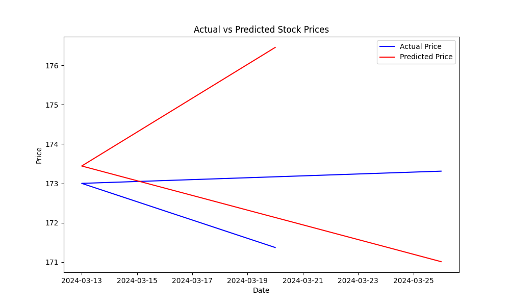
The Mean Squared Error (MSE) helps measure the prediction error of the model. The lower the MSE, the better the model's predictions. To visualize how well the model predicts stock prices, plot the actual vs. predicted prices:

import matplotlib.pyplot as plt

# Plot actual vs predicted prices
plt.figure(figsize=(10, 6))
plt.plot(y_test.index, y_test, label='Actual Price', color='blue')
plt.plot(y_test.index, y_pred, label='Predicted Price', color='red')
plt.title('Actual vs Predicted Stock Prices')
plt.xlabel('Date')
plt.ylabel('Price')
plt.legend()
plt.show()

This plot will help you visually assess the model’s performance, showing how close the predicted values are to the actual stock prices.

Full code:

import matplotlib.pyplot as plt
from sklearn.metrics import mean_squared_error
from sklearn.ensemble import RandomForestRegressor
from sklearn.model_selection import train_test_split
import yfinance as yf

# Fetch data for Apple (AAPL) from Yahoo Finance
data = yf.download('AAPL', start='2024-01-01', end='2024-04-01')
print(data.head())  # View the first few rows of the dataset

# Calculate Simple Moving Averages (SMA)
data['SMA_20'] = data['Close'].rolling(window=20).mean()
data['SMA_50'] = data['Close'].rolling(window=50).mean()

# Calculate Exponential Moving Averages (EMA)
data['EMA_20'] = data['Close'].ewm(span=20, adjust=False).mean()

# Calculate Relative Strength Index (RSI)
delta = data['Close'].diff(1)
gain = delta.where(delta > 0, 0)
loss = -delta.where(delta < 0, 0)
avg_gain = gain.rolling(window=14).mean()
avg_loss = loss.rolling(window=14).mean()
rs = avg_gain / avg_loss
data['RSI'] = 100 - (100 / (1 + rs))

# Drop rows with NaN values (due to moving averages and RSI)
data = data.dropna()

# Define the target variable as the next day's closing price
data['Target'] = data['Close'].shift(-1)

# Drop the last row, which has NaN in the 'Target' column
data = data.dropna(subset=['Target'])

# Feature set (SMA, EMA, RSI)
X = data[['SMA_20', 'SMA_50', 'EMA_20', 'RSI']]
y = data['Target']

# Split into training and testing data
X_train, X_test, y_train, y_test = train_test_split(
    X, y, test_size=0.2, random_state=42)

# Initialize and train the model
model = RandomForestRegressor(n_estimators=100, random_state=42)
model.fit(X_train, y_train)

# Predict on the test set
y_pred = model.predict(X_test)

# Evaluate the model using Mean Squared Error (MSE)
mse = mean_squared_error(y_test, y_pred)
print(f"Mean Squared Error: {mse}")


# Plot actual vs predicted prices
plt.figure(figsize=(10, 6))
plt.plot(y_test.index, y_test, label='Actual Price', color='blue')
plt.plot(y_test.index, y_pred, label='Predicted Price', color='red')
plt.title('Actual vs Predicted Stock Prices')
plt.xlabel('Date')
plt.ylabel('Price')
plt.legend()
plt.show()

7. Enhancing the Model

Now that you’ve built a basic model, there are several ways to improve its accuracy:

• Use Additional Features: Include more technical indicators, sentiment analysis data from news and social media, or even macroeconomic variables.

• Advanced Machine Learning Models: Try more sophisticated algorithms such as XGBoost, Gradient Boosting Machines (GBM), or Deep Learning models like LSTM for better performance on time-series data.

• Hyperparameter Tuning: Optimize model parameters using techniques like GridSearchCV or RandomSearchCV to find the best model configuration.

• Feature Selection: Use techniques like Recursive Feature Elimination (RFE) to identify the most important features contributing to predictions.

By continuously refining your model, incorporating more data, and experimenting with different algorithms, you can improve the predictive power of your stock market trend prediction model.

Next Steps

• Experiment with additional technical indicators and data sources.

• Try out different machine learning algorithms (e.g., LSTMs for deep learning).

• Backtest your model by simulating trades using historical data.

• Keep refining and optimizing your model based on feedback from real-world performance.