NS&I Premium Bonds: Insights from a Monte Carlo Experiment

In Part 1 of this series, we explored the characteristics of NS&I Premium Bonds and created a function to simulate the results of a single monthly prize draw for a given bond holding. In Part 2, we built a Monte Carlo experiment, simulated 6 million prize draws, loaded the results into a Polars dataframe, and saved it in parquet format. Now, we are ready to analyse this data to understand the likely returns from Premium Bonds under various scenarios.

Preliminary Prize Analysis

Let's begin by loading the data:

df = pl.read_parquet('premium_bond_6M_sim_202408.parquet')

As a reminder, this is a dataframe with 26.6 million rows, each corresponding to a prize won during one of the 6 million simulations. The first thing we should do is examine the distribution of prizes won to ensure this is consistent with the published figures used to construct the simulation function. This can be achieved using the group_by method, aggregating by prize frequency and expressing as a percentage of the total prizes.

df_prizes = df.group_by('prize').agg(
    pl.col('prize').len().alias('frequency')).sort('prize').with_columns(
        (pl.col('frequency')*100/len(df)).alias('percent').round(2))

with pl.Config(tbl_rows=-1):
    print('Prize distribution')
    print(df_prizes)

Prize distribution
shape: (11, 3)
┌─────────┬───────────┬─────────┐
│ prize   ┆ frequency ┆ percent │
│ ---     ┆ ---       ┆ ---     │
│ i32     ┆ u32       ┆ f64     │
╞═════════╪═══════════╪═════════╡
│ 25      ┆ 7095960   ┆ 24.85   │
│ 50      ┆ 10542024  ┆ 36.92   │
│ 100     ┆ 10546944  ┆ 36.94   │
│ 500     ┆ 262608    ┆ 0.92    │
│ 1000    ┆ 88998     ┆ 0.31    │
│ 5000    ┆ 8502      ┆ 0.03    │
│ 10000   ┆ 4386      ┆ 0.02    │
│ 25000   ┆ 1692      ┆ 0.01    │
│ 50000   ┆ 918       ┆ 0.0     │
│ 100000  ┆ 438       ┆ 0.0     │
│ 1000000 ┆ 12        ┆ 0.0     │
└─────────┴───────────┴─────────┘

The context manager with pl.Config(tbl_rows=-1) configures Polars to display all table rows. After grouping the dataframe by prize and counting the occurrences of each, the observed prize frequencies can be compared to the published rates.

For £50 and £100 prizes, the observed frequencies were within an acceptable margin of the expected 36.92%. Similarly, the £25 prize frequency of 24.87% aligned with the published rate.

However, for the £1 million jackpot, we observed a win rate of 1 in 2.38 million, which is 20% higher than the expected 1 in 2.97 million. This discrepancy is not unexpected due to the stochastic nature of the Monte Carlo method, particularly when dealing with rare events. To obtain more consistent results, an even larger number of simulations would be required.

Real-world Application

In order to apply the data to real-world scenarios involving different bond holding size and duration, it is necessary to perform a groupby on the simulation number and apply a filter on the winning bond number before using the agg method to obtain the sum of prizes won.

A challenge arises because the dataframe only contains data for simulations with at least one prize. This is demonstrated by looking at the shape of the resultant dataframe:

In[1]: df.group_by(pl.col('sim')).agg(pl.sum('prize')).shape
Out[1]: (5_947_776, 2)

There are only 5,947,776 rows instead of the expected 6 million. This implies that 52,224 simulations had no winning bonds. When grouping the data, some groups might contain only these missing simulations, leading to gaps in the resultant dataframe.

To address this, we create a complete dataframe with all possible simulation groups. Then, we left join the grouped dataframe on the simulation group and fill any missing values with zero. This ensures that all simulations, including those without prizes, are represented in the results:

all_simulations = pl.DataFrame({'sim_group': range(num_groups)},
                                   schema={'sim_group': pl.Int32})

result_df = all_simulations.join(grouped_df, on='sim_group', how='left')
result_df = result_df.fill_null(0)

The number of groups is calculated as num_groups = (6_000_000 + holding_span - 1) // holding_span, where holding_span is the number of months the bonds are held. If the six million simulations are not evenly divisible by the holding span, the last group is incomplete and should be excluded from the analysis. Therefore, num_groups is reduced by 1 before creating the all_simulations dataframe.

if 6_000_000 % holding_span:
    grouped_df = grouped_df.filter(
        pl.col('sim_group').mod(num_groups) != num_groups - 1)
    num_groups -= 1

All that remains is to define the grouped_df dataframe and encapsulate alongside the other code in a convenient function:

def group_df(df: pl.DataFrame, holding_size: int = 100_000,
             holding_span: int = 1) -> pl.DataFrame:
    """ Groups df into simulation groups according to the holding_span in months
        and filters bonds to the holding_size to produce a dataframe of total
        winnings for each sim_group
    """

    # Calculate number of required groups padding with holding_span-1 for
    # remainder items if holding_span is not a factor of 6_000_000
    num_groups = (6_000_000 + holding_span - 1) // holding_span

    # Build a lazy query filtering on bonds within holding_size and grouping
    # into num_groups to determine the total prizes won in each grouped sim
    q = (
        df.lazy()
        .filter(df['bond'] < holding_size)
        .group_by(pl.col('sim').mod(num_groups).alias('sim_group'))
        .agg(pl.sum('prize').alias('total_won'))
    )
    grouped_df = q.collect()

    # Remove last partial group if total sims is not divisible by holding_span
    if 6_000_000 % holding_span:
        grouped_df = grouped_df.filter(
            pl.col('sim_group').mod(num_groups) != num_groups - 1)
        num_groups -= 1

    # Fill in any gaps created by sims with no prizes
    all_simulations = pl.DataFrame({'sim_group': range(num_groups)},
                                   schema={'sim_group': pl.Int32})

    result_df = all_simulations.join(grouped_df, on='sim_group', how='left')
    result_df = result_df.fill_null(0)

    return result_df

To analyse winnings from holding 50,000 Premium Bonds over 12 monthly draws, we can use the following code:

In[2]: group_df(df, 50_000, 12).describe()
Out[2]: 
shape: (9, 3)
┌────────────┬───────────────┬─────────────┐
│ statistic  ┆ sim_group     ┆ total_won   │
│ ---        ┆ ---           ┆ ---         │
│ str        ┆ f64           ┆ f64         │
╞════════════╪═══════════════╪═════════════╡
│ count      ┆ 500000.0      ┆ 500000.0    │
│ null_count ┆ 0.0           ┆ 0.0         │
│ mean       ┆ 249999.5      ┆ 2189.7072   │
│ std        ┆ 144337.711635 ┆ 4899.286306 │
│ min        ┆ 0.0           ┆ 0.0         │
│ 25%        ┆ 125000.0      ┆ 1350.0      │
│ 50%        ┆ 250000.0      ┆ 1800.0      │
│ 75%        ┆ 374999.0      ┆ 2400.0      │
│ max        ┆ 499999.0      ┆ 305475.0    │
└────────────┴───────────────┴─────────────┘

As shown, the mean return in this scenario is just over £2,189 (4.38%), which is close to the published prize rate. However, the median return, representing average luck, is only £1,800 (3.6%), about 80% of the prize rate. This might be surprising to many Premium Bond holders, emphasising the importance of modelling the returns.

The previous analysis raises the question: how do holding size and holding span affect the median return? We will now explore these relationships:

Size Matters

To examine the impact of holding size on returns, we define the function get_data_holding_sizes. This function calls group_df with different holding sizes and pivots the data into a table of winnings versus holding size:

def get_data_holding_sizes(df: pl.DataFrame, holding_span: int = 1
                           ) -> pl.DataFrame:
    """ Calls group_df for a specified list of holding sizes and the provided
        holding_span, then pivots the data into a dataframe of holding size vs
        total_won for each sim_group
    """
    size_values = [500, 1_000, 2_000, 5_000, 10_000, 20_000, 50_000, 100_000]

    data = [[size, group_df(df, size, holding_span)]
            for size in size_values]

    pivoted_data = [
        100*12/holding_span/size*group['total_won'].alias(str(size))
        for size, group in data]

    return pl.DataFrame().with_columns(pivoted_data)

By applying this function to various holding sizes over 6 months and using the describe method, we obtain the following table:

[In 3]: stats = pl.DataFrame(pivoted_data[0].describe()['statistic']).with_columns(
   ...:    [col.describe()['value'].round(2).alias(col.name)
   ...:     for col in pivoted_data])

[In 4]: with pl.Config(tbl_cols=-1):
   ...:    print(stats)
[Out 4]:
shape: (9, 9)
┌────────────┬─────────┬─────────┬─────────┬────────┬────────┬────────┬───────┬────────┐
│ statistic  ┆ 500     ┆ 1000    ┆ 2000    ┆ 5000   ┆ 10000  ┆ 20000  ┆ 50000 ┆ 100000 │
│ ---        ┆ ---     ┆ ---     ┆ ---     ┆ ---    ┆ ---    ┆ ---    ┆ ---   ┆ ---    │
│ str        ┆ f64     ┆ f64     ┆ f64     ┆ f64    ┆ f64    ┆ f64    ┆ f64   ┆ f64    │
╞════════════╪═════════╪═════════╪═════════╪════════╪════════╪════════╪═══════╪════════╡
│ count      ┆ 1e6     ┆ 1e6     ┆ 1e6     ┆ 1e6    ┆ 1e6    ┆ 1e6    ┆ 1e6   ┆ 1e6    │
│ null_count ┆ 0.0     ┆ 0.0     ┆ 0.0     ┆ 0.0    ┆ 0.0    ┆ 0.0    ┆ 0.0   ┆ 0.0    │
│ mean       ┆ 4.4     ┆ 4.4     ┆ 4.3     ┆ 4.4    ┆ 4.4    ┆ 4.4    ┆ 4.4   ┆ 4.4    │
│ std        ┆ 101.0   ┆ 64.8    ┆ 40.1    ┆ 32.6   ┆ 24.0   ┆ 16.3   ┆ 10.3  ┆ 11.7   │
│ min        ┆ 0.0     ┆ 0.0     ┆ 0.0     ┆ 0.0    ┆ 0.0    ┆ 0.0    ┆ 0.0   ┆ 0.3    │
│ 25%        ┆ 0.0     ┆ 0.0     ┆ 0.0     ┆ 0.0    ┆ 1.0    ┆ 2.0    ┆ 2.7   ┆ 3.0    │
│ 50%        ┆ 0.0     ┆ 0.0     ┆ 0.0     ┆ 2.0    ┆ 3.0    ┆ 3.5    ┆ 3.6   ┆ 3.8    │
│ 75%        ┆ 0.0     ┆ 0.0     ┆ 5.0     ┆ 6.0    ┆ 5.5    ┆ 5.0    ┆ 4.8   ┆ 4.7    │
│ max        ┆ 40000.0 ┆ 20000.0 ┆ 10030.0 ┆ 8001.0 ┆ 4022.0 ┆ 2011.0 ┆ 810.2 ┆ 4006.9 │
└────────────┴─────────┴─────────┴─────────┴────────┴────────┴────────┴───────┴────────┘

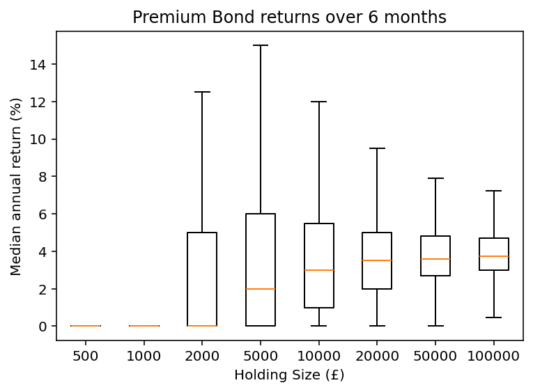
While the mean return is consistently around 4.4%, smaller holdings have a much lower probability of winning anything. The median return steadily increases with holding size, reaching 3.8% for a couple sharing £100,000.

The following chart visualises this relationship:

plt.boxplot(pivoted_data,
    labels=[s.name for s in pivoted_data], showfliers=False)
plt.xlabel("Holding Span (months)")
plt.ylabel("Median annual return (%)")
plt.title("Premium Bond returns over 6 months")

As shown, small holdings over short periods have a low probability of significant returns. The distribution of outcomes becomes narrower and the median return improves with larger holdings, but even the maximum holding size falls short of the published prize rate.

Patience is a Virtue

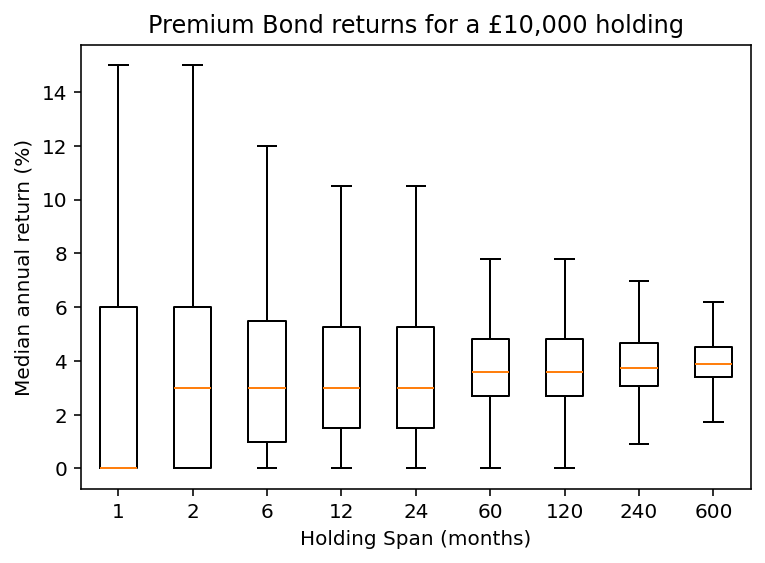
To explore the impact of holding span, we conduct a similar analysis using varying time periods. For example, the equivalent distribution for a £10,000 holding over varying periods of time shown below.

Return statistics for various holding spans for 10,000 bonds
shape: (9, 10)
┌──────────┬─────────┬────────┬────────┬─────────┬─────────┬─────────┬─────────┬─────────┬─────────┐
│ statisti ┆ 1       ┆ 2      ┆ 6      ┆ 12      ┆ 24      ┆ 60      ┆ 120     ┆ 240     ┆ 600     │
│ c        ┆ ---     ┆ ---    ┆ ---    ┆ ---     ┆ ---     ┆ ---     ┆ ---     ┆ ---     ┆ ---     │
│ ---      ┆ f64     ┆ f64    ┆ f64    ┆ f64     ┆ f64     ┆ f64     ┆ f64     ┆ f64     ┆ f64     │
│ str      ┆         ┆        ┆        ┆         ┆         ┆         ┆         ┆         ┆         │
╞══════════╪═════════╪════════╪════════╪═════════╪═════════╪═════════╪═════════╪═════════╪═════════╡
│ count    ┆ 6e6     ┆ 3e6    ┆ 1e6    ┆ 500000. ┆ 250000. ┆ 100000. ┆ 50000.0 ┆ 25000.0 ┆ 10000.0 │
│          ┆         ┆        ┆        ┆ 0       ┆ 0       ┆ 0       ┆         ┆         ┆         │
│ null_cou ┆ 0.0     ┆ 0.0    ┆ 0.0    ┆ 0.0     ┆ 0.0     ┆ 0.0     ┆ 0.0     ┆ 0.0     ┆ 0.0     │
│ nt       ┆         ┆        ┆        ┆         ┆         ┆         ┆         ┆         ┆         │
│ mean     ┆ 4.38    ┆ 4.38   ┆ 4.38   ┆ 4.38    ┆ 4.38    ┆ 4.38    ┆ 4.38    ┆ 4.38    ┆ 4.38    │
│ std      ┆ 45.49   ┆ 32.17  ┆ 23.97  ┆ 22.74   ┆ 22.74   ┆ 10.15   ┆ 10.15   ┆ 7.17    ┆ 4.53    │
│ min      ┆ 0.0     ┆ 0.0    ┆ 0.0    ┆ 0.0     ┆ 0.0     ┆ 0.0     ┆ 0.0     ┆ 0.6     ┆ 1.59    │
│ 25%      ┆ 0.0     ┆ 0.0    ┆ 1.0    ┆ 1.5     ┆ 1.5     ┆ 2.7     ┆ 2.7     ┆ 3.08    ┆ 3.39    │
│ 50%      ┆ 0.0     ┆ 3.0    ┆ 3.0    ┆ 3.0     ┆ 3.0     ┆ 3.6     ┆ 3.6     ┆ 3.75    ┆ 3.9     │
│ 75%      ┆ 6.0     ┆ 6.0    ┆ 5.5    ┆ 5.25    ┆ 5.25    ┆ 4.8     ┆ 4.8     ┆ 4.65    ┆ 4.53    │
│ max      ┆ 12060.0 ┆ 6031.5 ┆ 4022.0 ┆ 3017.25 ┆ 3017.25 ┆ 604.65  ┆ 604.65  ┆ 305.25  ┆ 124.47  │
└──────────┴─────────┴────────┴────────┴─────────┴─────────┴─────────┴─────────┴─────────┴─────────┘

For longer holding periods, the range of outcomes again converges. A £10,000 holding over 50 years generates a median return of 3.9%, which is 88% of the published prize rate.

Combined Analysis

To explore the combined effects of holding size and span, we can create a function to generate a table of rates:

def grouped_matrix(df: pl.DataFrame) -> pl.DataFrame:
    """ Calls group_df for a specified list of holding sizes and spans,
        then pivots the data into a dataframe of dataframes holding size vs
        holding_span
    """
    size_values = [500, 1_000, 2_000, 5_000, 10_000, 20_000, 50_000, 100_000]
    span_values = [1, 2, 6, 12, 24, 60, 120, 240, 600]

    data = [[size, span, group_df(df, size, span)]
            for size in size_values for span in span_values]

    matrix_df = pl.DataFrame(data, schema=["size", "span", "dataframe"],
                             orient='row')

    return matrix_df

The function returns a dataframe of dataframes, from which we can extract a dataframe of return rates:

def median_rate_matrix(matrix_df: pl.DataFrame) -> pl.DataFrame:
    """ Calculates median return percentage for the matrix_df obtained from
        grouped_matrix
    """
    median_prizes = [x.describe().filter(
        pl.col('statistic') == '50%')[0, 2] for x in matrix_df['dataframe']]

    # Create a new DataFrame using the median prizes
    rate_df = matrix_df['size', 'span'].with_columns(
        rate=pl.Series(median_prizes)/pl.col('size')/pl.col('span')*12*100)

    return rate_df

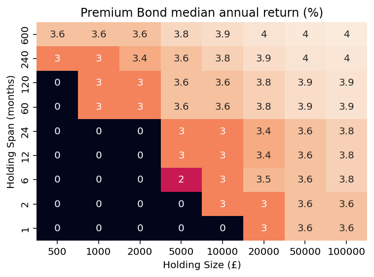
This allows us to generate a table of median returns, both as a percentage rate and as a percentage of the published prize rate.

Median return (%) for various holding sizes and spans
shape: (9, 9)
┌──────┬─────┬──────┬───────┬──────┬───────┬───────┬───────┬────────┐
│ span ┆ 500 ┆ 1000 ┆ 2000  ┆ 5000 ┆ 10000 ┆ 20000 ┆ 50000 ┆ 100000 │
│ ---  ┆ --- ┆ ---  ┆ ---   ┆ ---  ┆ ---   ┆ ---   ┆ ---   ┆ ---    │
│ i64  ┆ f64 ┆ f64  ┆ f64   ┆ f64  ┆ f64   ┆ f64   ┆ f64   ┆ f64    │
╞══════╪═════╪══════╪═══════╪══════╪═══════╪═══════╪═══════╪════════╡
│ 1    ┆ 0.0 ┆ 0.0  ┆ 0.0   ┆ 0.0  ┆ 0.0   ┆ 3.0   ┆ 3.6   ┆ 3.6    │
│ 2    ┆ 0.0 ┆ 0.0  ┆ 0.0   ┆ 0.0  ┆ 3.0   ┆ 3.0   ┆ 3.6   ┆ 3.6    │
│ 6    ┆ 0.0 ┆ 0.0  ┆ 0.0   ┆ 2.0  ┆ 3.0   ┆ 3.5   ┆ 3.6   ┆ 3.75   │
│ 12   ┆ 0.0 ┆ 0.0  ┆ 0.0   ┆ 3.0  ┆ 3.0   ┆ 3.375 ┆ 3.6   ┆ 3.75   │
│ 24   ┆ 0.0 ┆ 0.0  ┆ 0.0   ┆ 3.0  ┆ 3.0   ┆ 3.375 ┆ 3.6   ┆ 3.75   │
│ 60   ┆ 0.0 ┆ 3.0  ┆ 3.0   ┆ 3.6  ┆ 3.6   ┆ 3.75  ┆ 3.9   ┆ 3.945  │
│ 120  ┆ 0.0 ┆ 3.0  ┆ 3.0   ┆ 3.6  ┆ 3.6   ┆ 3.75  ┆ 3.9   ┆ 3.945  │
│ 240  ┆ 3.0 ┆ 3.0  ┆ 3.375 ┆ 3.6  ┆ 3.75  ┆ 3.9   ┆ 3.96  ┆ 3.9975 │
│ 600  ┆ 3.6 ┆ 3.6  ┆ 3.6   ┆ 3.84 ┆ 3.9   ┆ 3.96  ┆ 4.008 ┆ 4.05   │
└──────┴─────┴──────┴───────┴──────┴───────┴───────┴───────┴────────┘
Median return as a percentage of the prize rate
shape: (9, 9)
┌──────┬─────┬──────┬──────┬──────┬───────┬───────┬───────┬────────┐
│ span ┆ 500 ┆ 1000 ┆ 2000 ┆ 5000 ┆ 10000 ┆ 20000 ┆ 50000 ┆ 100000 │
│ ---  ┆ --- ┆ ---  ┆ ---  ┆ ---  ┆ ---   ┆ ---   ┆ ---   ┆ ---    │
│ i64  ┆ i16 ┆ i16  ┆ i16  ┆ i16  ┆ i16   ┆ i16   ┆ i16   ┆ i16    │
╞══════╪═════╪══════╪══════╪══════╪═══════╪═══════╪═══════╪════════╡
│ 1    ┆ 0   ┆ 0    ┆ 0    ┆ 0    ┆ 0     ┆ 68    ┆ 82    ┆ 82     │
│ 2    ┆ 0   ┆ 0    ┆ 0    ┆ 0    ┆ 68    ┆ 68    ┆ 82    ┆ 82     │
│ 6    ┆ 0   ┆ 0    ┆ 0    ┆ 45   ┆ 68    ┆ 80    ┆ 82    ┆ 85     │
│ 12   ┆ 0   ┆ 0    ┆ 0    ┆ 68   ┆ 68    ┆ 77    ┆ 82    ┆ 85     │
│ 24   ┆ 0   ┆ 0    ┆ 0    ┆ 68   ┆ 68    ┆ 77    ┆ 82    ┆ 85     │
│ 60   ┆ 0   ┆ 68   ┆ 68   ┆ 82   ┆ 82    ┆ 85    ┆ 89    ┆ 90     │
│ 120  ┆ 0   ┆ 68   ┆ 68   ┆ 82   ┆ 82    ┆ 85    ┆ 89    ┆ 90     │
│ 240  ┆ 68  ┆ 68   ┆ 77   ┆ 82   ┆ 85    ┆ 89    ┆ 90    ┆ 91     │
│ 600  ┆ 82  ┆ 82   ┆ 82   ┆ 87   ┆ 89    ┆ 90    ┆ 91    ┆ 92     │
└──────┴─────┴──────┴──────┴──────┴───────┴───────┴───────┴────────┘

Even with a large holding over a lifetime, an individual with average luck would achieve around 90% of the published prize rate. When comparing Premium Bonds to conventional savings, it's therefore essential to consider factors beyond the headline rate.

A heatmap can effectively visualise this data. The following code generates a heatmap for the rate of return; to visualise the percentage of the prize rate, we first divide the values in rate_df by the prize rate using pct_df = rate_df.with_columns((pl.col('rate')/0.044).round(0).cast(pl.Int16)).

pivoted_rate_df = rate_df.pivot('size', index='span', values='rate')
pd_df_piv = pivoted_rate_df.to_pandas().set_index('span').iloc[::-1, :]
sns.heatmap(pd_df_piv, annot=True, cbar=False)
plt.xlabel("Holding Size (£)")
plt.ylabel("Holding Span (months)")
plt.title("Premium Bond median annual return (%)")

Conclusion

The analysis of NS&I Premium Bonds using the Monte Carlo experiment performed in Part 2 of this series has provided valuable insights.

We verified the accuracy of the simulated data against the published prize distributions and explored its real-world applicability. Through data imputation, we addressed the challenge of simulations with no winning bonds, ensuring data consistency.

Analysing holding size and duration revealed that while the mean return aligns closely with the published prize rate, the median return often falls short. This emphasises the importance of modelling to understand the full range of potential outcomes. The combined analysis of holding size and span further demonstrated that even with large holdings over extended periods, the median return remains below the published rate.

These findings underscore the need for Premium Bond holders to consider factors beyond the headline rate when evaluating their investment.

The complete code used in this series of articles is available in the premium_bond_sim repository on my GitHub page for reference and further exploration. The analysis can be re-run whenever NS&I changes the winning odds and prize distribution, as they occasionally do.