How to Create a Pneumonia Detection Model with Convolutional Neural Networks

In this article, I share my journey of implementing a Pneumonia detection model using convolutional neural networks with PyTorch. Starting from dataset preparation and transformation, I guide you through the process of splitting the dataset, defining and implementing the CNN architecture, and the training-validation workflow. Key concepts such as convolution, activation, pooling, and backpropagation are explained. I also touch on preventing overfitting and model evaluation, with code snippets and tips on saving the best-performing model. This hands-on project helped me better understand the workings of neural networks and offers a roadmap for improving the implementation.

Introduction

After learning about convolutional neural networks, I wanted to implement something on my own. The implementation is very improvable but helped me better understand how things work. In the following article, I'll share my thoughts on this project along with the code and some ways to improve it.

Dataset Preparation

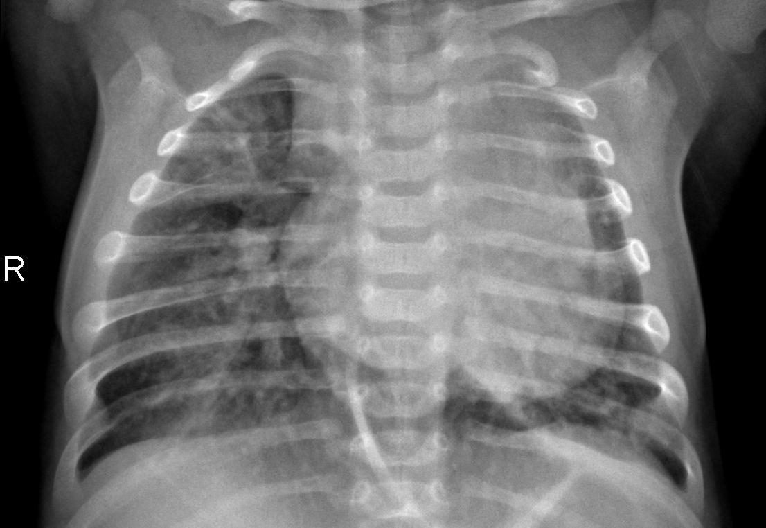
The dataset contains 5,863 X-ray images (JPEG) of 2 categories (Pneumonia/Normal) in black and white and is available here.

My first step was downloading and properly formatting the dataset. The dataset can be downloaded directly from Kaggle using an API key, but I chose to download the 2 GB file and run everything locally.

I then proceeded to transform it to the proper format for Pytorch and load it in the dataset variable. This is done here.

# Define transformations
transform = transforms.Compose([
    transforms.Resize((64,64)),  # Resize images to 64x64 pixels
    transforms.Grayscale(num_output_channels=1),  # Convert images to grayscale
    transforms.ToTensor(),        # Convert images to PyTorch tensors
])

# Load the dataset from the file system
dataset = datasets.ImageFolder(root='dataset', transform=transform)

The goal is to standardize the input format for the neural network and reduce computational load.

This is done in the transform, which is defined and then applied to every image loaded in the dataset variable. As the images of the dataset vary in size they are all reduced in size to 64 by 64 using Resize, which loses information and is not optimal but higher resolution would make it hard to train on my machine.

As you may know, the standard way of representing images is RGB, meaning that for each pixel of the images we have the value of the intensity of red, green, and blue (the primary colors) composing the pixel's color. These values are stored in three matrices.

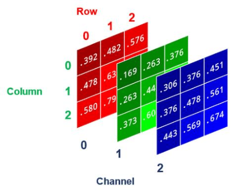
if we look at our dataset we can see that the images are in black and white. This means that we only need one matrix to represent the intensity

This representation is called grayscale and helps us represent black-and-white images using a third of the resources without losing any information. We implement this idea using transform.Grayscale. Finally, we convert the final data in pytorch tensors to store it efficiently. I could also have normalized the values by dividing them by 255 (The values range from 0 to 255 cause it is the biggest value you can store in a byte).

Splitting the Dataset

The next step was to split the dataset into test, train, and validation sets because I only used 3000 images and not the whole dataset. The idea behind this is that you want to get a model that is able to generalize, meaning that it understands patterns rather than learning by heart. To check this we will split the dataset into training and test sets. Meaning that the model will be tested on images it has never seen. We also add a validation set to check for overfitting.

The Data loader is used to process the images in blocks for faster training. The images are shuffled so as not to make the model learn some false pattern.

# Optionally, split the dataset into training and validation sets
train_size = int(0.8 * len(dataset))
valid_size = len(dataset) - train_size
train_dataset, valid_dataset = torch.utils.data.random_split(dataset, [train_size, valid_size])

# Create DataLoader instances for training and validation
train_loader = DataLoader(train_dataset, batch_size=32, shuffle=True)
valid_loader = DataLoader(valid_dataset, batch_size=32)

During the training, we will compare the model's performance on the training data and on the validation data which he has not seen during the training. The training should stop when the validation loss goes up because the validation loss going up means that the model becomes too specialized on the training dataset set and, hence less useful for real-world applications.

Overfitting can be visualized as a student who tries to remember by heart all the answers to his upcoming math test and thus will not be able to answer if there is a slight twist to the questions or if the numbers changed. It's the same thing for your model, you want it to have predictive power on new questions of the same type rather than just remembering all the answers for the training set.

Model Architecture

Now that we have preprocessed the data let's go on to discuss the model's architecture.

class BinaryClassifierCNN(nn.Module):
    def __init__(self):
        super(BinaryClassifierCNN, self).__init__()
        self.conv1 = nn.Conv2d(1, 32, kernel_size=2, stride=2, padding=0)  # Le 1 indique un seul canal d'entrée (grayscale)
        self.pool = nn.MaxPool2d(kernel_size=2, stride=2, padding=0)
        self.conv2 = nn.Conv2d(32, 64, kernel_size=3, stride=1, padding=1)
        self.fc1 = nn.Linear(4096, 512)
        self.fc2 = nn.Linear(512, 1)
        self.flatten = nn.Flatten()

    def forward(self, x):
        x = self.pool(F.relu(self.conv1(x)))
        x = self.pool(F.relu(self.conv2(x)))
        x = self.flatten(x)
        x = F.relu(self.fc1(x))
        x = torch.sigmoid(self.fc2(x))  # Utilisez sigmoid à la fin pour la classification binaire
        return x

# Initialiser le modèle
model = BinaryClassifierCNN()

The architecture is very simple but can be scaled if you have access to more computing power. Let's break it down: first, there are 2 convolutional layers as illustrated in the orange box.

This block is composed of a convolution, followed by an application of the Relu function and then some pooling action.

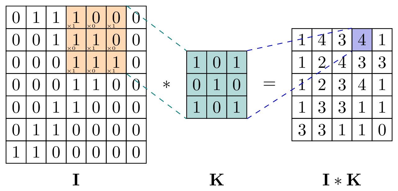
The convolution as shown below is a filter that goes through the image represented as a matrix on the left, creating a new transformed matrix. We get the values of the new matrix by adding up the multiplication of the values at the same positions.

The values of the filter are set at random at first and will evolve as the model is learning. The idea is to capture one specific feature of the image with each filter. We can play with the number of filters applied, the size of the filter (kernel size), how fast the filter goes through the matrix (stride), and padding (adding some 0 to keep the same matrix size)

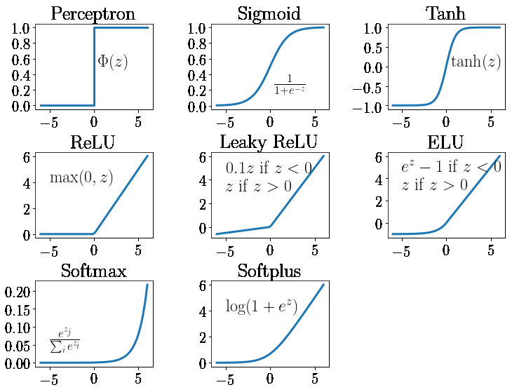
After this, we pass the result into an activation function as shown below. The point is to introduce some nonlinearity to help the model learn some more complex features that can't be represented by linear functions. I chose to work with Relu but I've heard that using Leaky Relu instead could improve the performances.

Finally, we end the block with a pooling action. The idea of pooling is to get rid of the noise and only keep the relevant information, which reduces the necessary computing power and improves accuracy. I chose to work with the max pooling which keeps the biggest local value as shown below.

I repeated this convolutional layer twice but you could increase the number of blocks and have more parameters for your model (which should increase the performance). I had some issues keeping track of the evolving sizes of the images after the convolution.

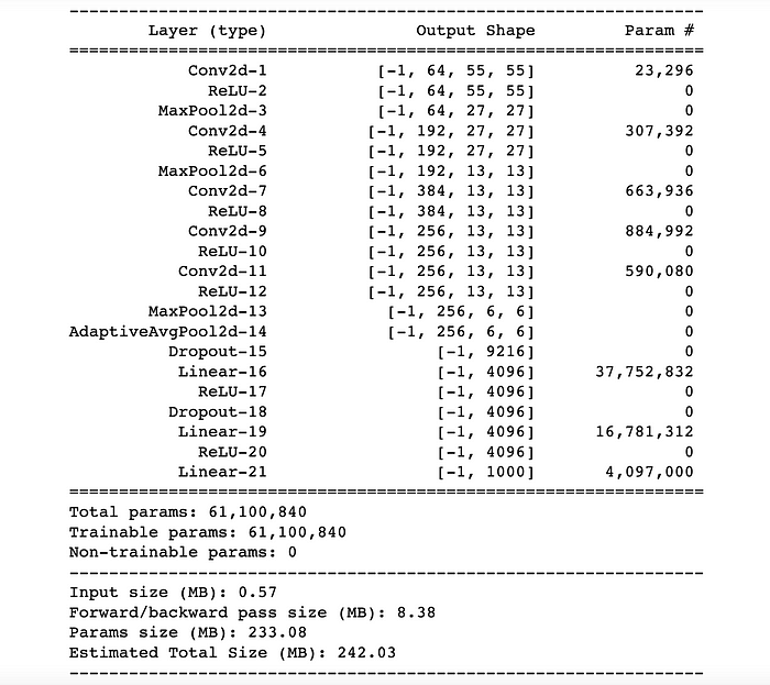
I ended up figuring it out using torch summary which prints out the sizes at each layer. The point is to make the output size match the next input size as this is a common (and annoying) error.

Later I was told that, another way of doing this is to compute the sizes using the following formula which can save some time:

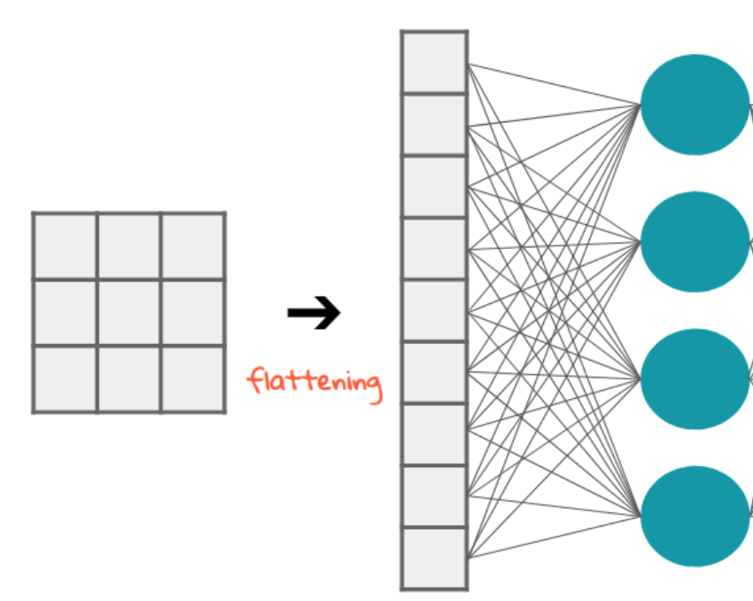
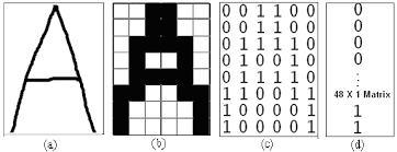
Having done our convolutions (as many as we chose to) we Flatten the result to get an array for the linear layer. Flattening the matrix means compressing the (same) information by diminishing the dimension.

Then we do a weighted sum of these values and put it into an activation function. I used Softmax because it directly gives me a probability, but using a Tanh and then normalizing it gives better results.

Training the Model

After this, we still need to figure out how the model actually learns.

What we have now is a model that takes an input(the X-ray), and makes computations with random weights with it, thus giving us a random output (the probability of having pneumonia).

We need to give our model some feedback on how it performed. This is done through the Loss function which quantifies how far the predicted result is from the real value. In my case, I use the Binary Cross Entropy Loss which works for classification tasks with two classes, which is our case (0 if healthy, 1 if sick).

$$BCE(y, yi ​ )=−(y⋅log( y ^ ​ )+(1−y)⋅log(1− yi ​ ))$$

Here y represents the real result, and yi is the predicted probability normalized by the the sample size N. The minus sign ensures that when p (the predicted probability) is close to 0 or 1, the loss remains positive and meaningful by counteracting the negative logarithms, as

$$log(p)→−∞ \hspace{5 mm} when\hspace{5 mm}p→0$$

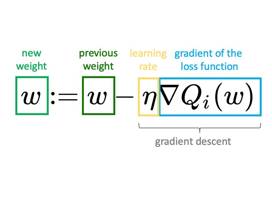
Now that we have our feedback we use it to improve our performance (we achieve that by adjusting the weights). This process is called backpropagation and is crucial in machine learning.

To improve the quality of our weights we start by figuring out how much each weight contributed to the final prediction. These contributions to the loss are called gradients.

The gradients of the loss function are computed with respect to each model parameter using the chain rule, which breaks down the gradient of a composed function into a product of simpler gradients. This allows us to determine the influence of each weight on the loss.

The gradients indicate both the direction and magnitude of the necessary adjustment to reduce the loss.

Once the gradients are computed, the model's parameters are updated to minimize the loss function. This update is usually performed using the gradient descent algorithm.

• 

By repeating this process over several iterations (called epochs in machine learning), the weights are adjusted to minimize the loss, thus training the model.

This is what is executed here: we make predictions in the Forward pass and update the weights during the backward pass, then I chose to evaluate the model using the validation loss, which is an average for all the images.

for epoch in range(num_epochs):
    model.train()  
    total_train_loss = 0.0
    for inputs, labels in train_loader:  # Assuming you have a DataLoader named train_loader
        # Forward pass
        y_pred = model.forward(inputs)
        y_pred = y_pred.squeeze() 
        labels = labels.float()  
        loss = criterion(y_pred,labels) 
        total_train_loss += loss.item()

        # Backward and optimize
        optimizer.zero_grad()
        loss.backward()  
        optimizer.step()  
      # Calculate average training loss for the epoch
    avg_train_loss = total_train_loss / len(train_loader)
    train_errors.append(avg_train_loss)

    # Validation
    model.eval()  # Set the model to evaluation mode
    total_val_loss = 0.0
    with torch.no_grad():  # disable gradient computation (more efficient and reduces memory usage)
        for images, labels in valid_loader:
            outputs = model(images)
            labels = labels.float()  # Ensure labels are floating-point for BCELoss

            # There's no need to squeeze the outputs as your last layer is a sigmoid, expected to work with BCELoss directly.
            # Just ensure that labels and outputs are of the same dimension.
            loss = criterion(outputs.squeeze(), labels)  # Compute the loss, ensuring output dimensions match labels

            total_val_loss += loss.item()

    # Calculate average validation loss for the epoch
    avg_val_loss = total_val_loss / len(valid_loader)
    val_errors.append(avg_val_loss)

    print(f'Epoch [{epoch+1}/{num_epochs}], Training Loss: {avg_train_loss:.4f}, Validation Loss: {avg_val_loss:.4f}')

A good thing to do is to save the weights of your model when it has improved (the validation loss has decreased) and to stop training when the validation loss has stopped improving for multiple epochs (is done with a patience counter and a condition to break).

 # Save model if validation loss has decreased
    if avg_val_loss < best_val_loss:
        print(f'Validation loss decreased ({best_val_loss:.4f} --> {avg_val_loss:.4f}). Saving model...')
        best_val_loss = avg_val_loss
        torch.save(model.state_dict(), 'Best_model.pth')
        patience_counter = 0  # Reset patience counter after improvement

With this, you should get a decreasing loss and increasing accuracy and be able to predict pneumonia with chest X-rays. Hopefully, you would have an accuracy curve looking like this:

I achieved results ranging from 67% to 85% accuracy by scaling the model—primarily through increasing the number of convolutional blocks, using a larger portion of the dataset, and extending the number of epochs (training iterations).

Experimenting with UNet architectures, which are widely used in medical imaging, could improve localization and segmentation of pneumonia-affected areas, would be an interesting idea. Additionally, Vision Transformers (ViTs) have been tested on the same dataset, and achieved an impressive 98% accuracy, suggesting that incorporating these advanced models could be a game-changer for this task.

Conclusion

Building a Pneumonia detection model using convolutional neural networks (CNNs) in PyTorch was a valuable learning experience. From dataset preparation and transformation to model architecture design and training, I gained a deeper understanding of how CNNs process and classify images. The project not only reinforced key concepts like convolution, activation functions, and backpropagation but also highlighted important strategies for handling overfitting and optimizing model performance.

While the model achieved reasonable accuracy, there is room for improvement—whether through experimenting with more complex architectures, tuning hyperparameters, or using techniques like data augmentation. Feel free to explore the full implementation on my GitHub, where I also tested a random forest model for comparison. I hope this proves useful in your learning journey and future projects!

If you found this article helpful and want to stay updated with more insightful content, consider subscribing to my newsletter where I document my progress on ongoing projects.