A Step by Step Guide to Principal Component Analysis (PCA) in Machine Learning
 Arbash Hussain
Introduction
Welcome back to the eighth blog post in our Machine Learning series! Today, we're diving into Principal Component Analysis (PCA), a powerful tool for dimensionality reduction. PCA simplifies complex datasets while keeping as much information as possible. By the end of this post, you'll understand how PCA works and why it works, with a clear mathematical intuition. As always, we will also implement this algorithm from scratch in Python.
Implementation code on my GitHub.
Why Do We Need Dimensionality Reduction?
When working with large datasets with many features (high-dimensional data), you may encounter issues like:
Overfitting: More features can make your model more complex, and it may start to "memorize" the training data rather than generalize from it.
Increased Computational Cost: More features mean your models take longer to train.
Redundancy: Many features might be correlated and essentially represent the same information.
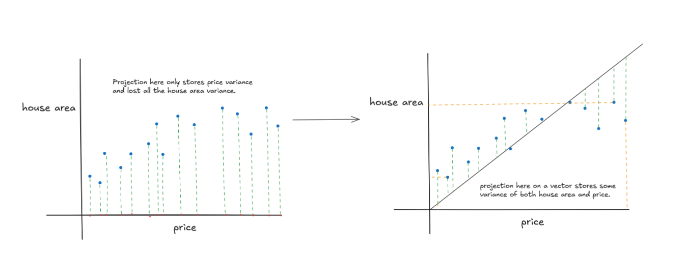
This is where PCA comes in—it reduces the dimensionality of our data by transforming it into a smaller set of uncorrelated variables, called principal components, while still retaining most of the original variance.

What is PCA?
PCA is a technique used to reduce the dimensionality of data by finding a new set of variables that are uncorrelated and ordered by the amount of variance they explain. These new variables, called principal components, are linear combinations of the original features.
Let’s get into the mathematical intuition behind PCA!
Mathematical Intuition of PCA
Mean Centering: First, we center our data by subtracting the mean of each feature. This step ensures that the data is aligned around the origin, which is necessary for the subsequent steps of PCA.
Mathematically, if we have data X with n features and m samples, we calculate the mean μ for each feature:
$$\mu_j = \frac{1}{m} \sum_{i=1}^{m} X_{ij}$$
Then, we subtract the mean from the original data:
$$X_{\text{centered}} = X - \mu$$
Covariance Matrix: After centering the data, the next step is to calculate the covariance matrix. The covariance matrix tells us how much each feature varies from the mean and how much two features vary together (i.e., how they are correlated).
Covariance between two features Xi and Xj is calculated as:
$$\text{Cov}(X_i, X_j) = \frac{1}{m-1} \sum_{k=1}^{m} (X_{k,i} - \mu_i)(X_{k,j} - \mu_j)$$
The covariance matrix for n features is an n x n matrix:
$$\text{Cov}(X) = \begin{pmatrix} \text{Cov}(X_1, X_1) & \text{Cov}(X_1, X_2) & \dots & \text{Cov}(X_1, X_n) \\ \text{Cov}(X_2, X_1) & \text{Cov}(X_2, X_2) & \dots & \text{Cov}(X_2, X_n) \\\ \vdots & \vdots & \ddots & \vdots \\ \text{Cov}(X_n, X_1) & \text{Cov}(X_n, X_2) & \dots & \text{Cov}(X_n, X_n) \end{pmatrix}$$
Why Do We Need the Covariance Matrix? The covariance matrix helps us understand the relationships between different features. If two features are highly correlated, they don’t provide unique information, and we may want to reduce this redundancy. PCA transforms the data into new features (principal components) that are uncorrelated.
Eigenvectors and Eigenvalues: After obtaining the covariance matrix, the next step is to find its eigenvectors and eigenvalues.
Eigenvectors represent directions (axes) in the feature space along which the data varies the most.
Eigenvalues represent the magnitude of the variance along these eigenvector directions.
For a matrix A, an eigenvector v and its corresponding eigenvalue λ are defined as:
$$Av = \lambda v$$
In simpler terms:
Eigenvectors show us the direction of the most variance in the data.
Eigenvalues tell us how much variance exists in each eigenvector’s direction.
Why Do We Need Eigenvectors and Eigenvalues? In PCA, the eigenvectors define the new set of axes (principal components), and the eigenvalues tell us how much variance each component captures. We sort the eigenvectors by their corresponding eigenvalues in descending order and select the top k eigenvectors that explain the most variance in the data. These top k eigenvectors form the principal components.
- Choosing Principal Components: After sorting the eigenvectors by their eigenvalues, we select the top k eigenvectors. These eigenvectors form the principal components, which are the new features that capture the most variance in the data.
Projecting Data onto Principal Components: Once we’ve chosen the principal components, we project the original data onto these new components to obtain a lower-dimensional representation.
Mathematically, if W is the matrix of the top k eigenvectors (principal components), we project the original data X onto these components by:
$$X_{\text{projected}} = X_{\text{centered}} \cdot W$$
Hyperparameters in PCA
- n_components: This is the main hyperparameter in PCA. It defines the number of principal components you want to keep. If you have 10 features, you might choose 2 components to reduce the dimensionality while retaining most of the variance.
Implementation Steps
The code is available on GitHub.
import numpy as np

# PCA Class
class PCA:

# Function 1: Initialize PCA Class
    def __init__(self, n_components):
        self.n_components = n_components  # Number of principal components to keep
        self.components = None  # To store the principal components
        self.mean = None  # To store the mean of the data

# Function 2: Fit the model
    def fit(self, X):
        # Mean centering
        self.mean = np.mean(X, axis=0)  # Calculate the mean of each feature
        X = X - self.mean  # Subtract the mean from the data to center it

        # Calculate the covariance matrix of the data
        cov = np.cov(X.T)

        # Compute the eigenvectors and eigenvalues
        eigenvectors, eigenvalues = np.linalg.eig(cov)

        # Sort eigenvectors by eigenvalues
        eigenvectors = eigenvectors.T  # Transpose the eigenvectors matrix for easier manipulation
        idxs = np.argsort(eigenvalues)[::-1]  # Sort eigenvalues in descending order
        eigenvalues = eigenvalues[idxs]  # Reorder eigenvalues
        eigenvectors = eigenvectors[idxs]  # Reorder eigenvectors accordingly

        # Store the top n principal components
        self.components = eigenvectors[:self.n_components]

# Function 3: Transform the data
    def transform(self, X):
        # Project data onto the principal components
        X = X - self.mean  # Subtract the mean to center the data again
        return np.dot(X, self.components.T)  # Perform the dot product to project the data onto the new components
Example
if __name__ == "__main__":
    import matplotlib.pyplot as plt
    from sklearn.datasets import load_iris

    data = load_iris()
    X = data.data
    y = data.target

    pca = PCA(2)
    pca.fit(X)
    X_projected = pca.transform(X)

    print("Shape of X:", X.shape)
    print("Shape of transformed X:", X_projected.shape)

    x1 = X_projected[:, 0]
    x2 = X_projected[:, 1]

    plt.scatter(
        x1, x2, c=y, edgecolor="none", alpha=0.8, cmap=plt.cm.get_cmap("viridis", 3)
    )

    plt.xlabel("PCA 1")
    plt.ylabel("PCA 2")
    plt.colorbar()
    plt.show()
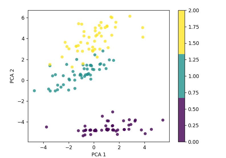
Output

Common Misconceptions about PCA
PCA loses important data: Not necessarily. PCA keeps the most important information while discarding the less significant parts.
PCA only works with numeric data: While PCA works best with numerical data, we can preprocess categorical data to use PCA.
When to apply PCA
High Dimensionality: When we have many features and want to reduce complexity.
Noise Reduction: PCA helps clean noisy data.
Visualization: PCA is often used to visualize high-dimensional data in 2D or 3D.
Advantages of PCA
Simplifies Complex Data: Reduces the number of features while retaining important information.
Improves Performance: Can speed up machine learning models by removing noise.
Helps with Visualization: Makes it easier to visualize high-dimensional data.
Disadvantages of PCA
Interpretability: The new features (principal components) are often hard to interpret.
Data Loss: While PCA aims to retain the most important information, some data loss is inevitable.
Affected by outliers: This can distort the principal components and affect the accuracy of the results.
Practical Applications
Image Compression: Reducing the size of image files while maintaining quality.
Genomics: Simplifying genetic data for easier analysis.
Finance: Reducing the number of variables in economic models.
Conclusion
I hope this guide is useful to you. If so, please like and follow. You can also check out my other blogs in my series on machine learning algorithms. Your feedback and engagement are highly appreciated, so feel free to share your thoughts or ask questions in the comments section.
Subscribe to my newsletter
Read articles from Arbash Hussain directly inside your inbox. Subscribe to the newsletter, and don't miss out.
Written by

Arbash Hussain
Arbash Hussain
I'm a Computer Science Engineer with a passion for data science and AI. My interest for computer science has motivated me to work with various tech stacks like Flutter, Next.js, React.js, Pygame and Unity. For data science projects, I've used tools like MLflow, AWS, Tableau, SQL, and MongoDB, and I've worked with Flask and Django to build data-driven applications. I'm always eager to learn and stay updated with the latest in the field. I'm looking forward to connecting with like-minded professionals and finding opportunities to make an impact through data and AI.