Face Recognition with Local Binary Patterns (LBPs) and OpenCV

Last Updated : 13 Sep, 2024

by Pranav Sirsufale

In this article, Face Recognition with Local Binary Patterns (LBPs) and OpenCV is discussed. Let’s start with understanding the logic behind performing face recognition using LBPs. A beginner-friendly explanation of LBPs is described below.

Understanding LBPH Algorithm:

Human beings perform face recognition automatically every day and practically with no effort.

Although it sounds like a very simple task for us, it has proven to be a complex task for a computer, as it has many variables that can impair the accuracy of the methods, for example: illumination variation, low resolution, occlusion, amongst other.

In computer science, face recognition is basically the task of recognizing a person based on its facial image. It has become very popular in the last two decades, mainly because of the new methods developed and the high quality of the current videos/cameras.

Note that face recognition is different of face detection:

Face Detection: it has the objective of finding the faces (location and size) in an image and probably extract them to be used by the face recognition algorithm.

Face Recognition: with the facial images already extracted, cropped, resized and usually converted to grayscale, the face recognition algorithm is responsible for finding characteristics which best describe the image.

The face recognition systems can operate basically in two modes:

Verification or authentication of a facial image: it basically compares the input facial image with the facial image related to the user which is requiring the authentication. It is basically a 1x1 comparison.

Identification or facial recognition: it basically compares the input facial image with all facial images from a dataset with the aim to find the user that matches that face. It is basically a 1xN comparison.

There are different types of face recognition algorithms, for example:

Eigenfaces (1991)

Local Binary Patterns Histograms (LBPH) (1996)

Fisherfaces (1997)

Scale Invariant Feature Transform (SIFT) (1999)

Speed Up Robust Features (SURF) (2006)

Each method has a different approach to extract the image information and perform the matching with the input image. However, the methods Eigenfaces and Fisherfaces have a similar approach as well as the SIFT and SURF methods.

Today we gonna talk about one of the oldest (not the oldest one) and more popular face recognition algorithms: Local Binary Patterns Histograms (LBPH).

Objective

The objective of this post is to explain the LBPH as simple as possible, showing the method step-by-step.

As it is one of the easier face recognition algorithms I think everyone can understand it without major difficulties.

Introduction

Local Binary Pattern (LBP) is a simple yet very efficient texture operator which labels the pixels of an image by thresholding the neighborhood of each pixel and considers the result as a binary number.

It was first described in 1994 (LBP) and has since been found to be a powerful feature for texture classification. It has further been determined that when LBP is combined with histograms of oriented gradients (HOG) descriptor, it improves the detection performance considerably on some datasets.

Using the LBP combined with histograms we can represent the face images with a simple data vector.

As LBP is a visual descriptor it can also be used for face recognition tasks, as can be seen in the following step-by-step explanation.

Step-by-Step

Now that we know a little more about face recognition and the LBPH, let’s go further and see the steps of the algorithm:

Parameters: the LBPH uses 4 parameters:

Radius: the radius is used to build the circular local binary pattern and represents the radius around the central pixel. It is usually set to 1.

Neighbors: the number of sample points to build the circular local binary pattern. Keep in mind: the more sample points you include, the higher the computational cost. It is usually set to 8.

Grid X: the number of cells in the horizontal direction. The more cells, the finer the grid, the higher the dimensionality of the resulting feature vector. It is usually set to 8.

Grid Y: the number of cells in the vertical direction. The more cells, the finer the grid, the higher the dimensionality of the resulting feature vector. It is usually set to 8.

2. Training the Algorithm: First, we need to train the algorithm. To do so, we need to use a dataset with the facial images of the people we want to recognize. We need to also set an ID (it may be a number or the name of the person) for each image, so the algorithm will use this information to recognize an input image and give you an output. Images of the same person must have the same ID. With the training set already constructed, let’s see the LBPH computational steps.

3. Applying the LBP operation: The first computational step of the LBPH is to create an intermediate image that describes the original image in a better way, by highlighting the facial characteristics. To do so, the algorithm uses a concept of a sliding window, based on the parameters radius and neighbors.

The image below shows this procedure:

Based on the image above, let’s break it into several small steps so we can understand it easily:

Suppose we have a facial image in grayscale.

We can get part of this image as a window of 3x3 pixels.

It can also be represented as a 3x3 matrix containing the intensity of each pixel (0~255).

Then, we need to take the central value of the matrix to be used as the threshold.

This value will be used to define the new values from the 8 neighbors.

For each neighbor of the central value (threshold), we set a new binary value. We set 1 for values equal or higher than the threshold and 0 for values lower than the threshold.

Now, the matrix will contain only binary values (ignoring the central value). We need to concatenate each binary value from each position from the matrix line by line into a new binary value (e.g. 10001101). Note: some authors use other approaches to concatenate the binary values (e.g. clockwise direction), but the final result will be the same.

Then, we convert this binary value to a decimal value and set it to the central value of the matrix, which is actually a pixel from the original image.

At the end of this procedure (LBP procedure), we have a new image which represents better the characteristics of the original image.

Note: The LBP procedure was expanded to use a different number of radius and neighbors, it is called Circular LBP.

It can be done by using bilinear interpolation. If some data point is between the pixels, it uses the values from the 4 nearest pixels (2x2) to estimate the value of the new data point.

4. Extracting the Histograms: Now, using the image generated in the last step, we can use the Grid X and Grid Y parameters to divide the image into multiple grids, as can be seen in the following image:

Based on the image above, we can extract the histogram of each region as follows:

[if !supportLists]· [endif]As we have an image in grayscale, each histogram (from each grid) will contain only 256 positions (0~255) representing the occurrences of each pixel intensity.

[if !supportLists]· [endif]Then, we need to concatenate each histogram to create a new and bigger histogram. Supposing we have 8x8 grids, we will have 8x8x256=16.384 positions in the final histogram. The final histogram represents the characteristics of the image original image.

The LBPH algorithm is pretty much it.

5. Performing the face recognition: In this step, the algorithm is already trained. Each histogram created is used to represent each image from the training dataset. So, given an input image, we perform the steps again for this new image and creates a histogram which represents the image.

So to find the image that matches the input image we just need to compare two histograms and return the image with the closest histogram.

We can use various approaches to compare the histograms (calculate the distance between two histograms), for example: euclidean distance, chi-square, absolute value, etc. In this example, we can use the Euclidean distance (which is quite known) based on the following formula:

So the algorithm output is the ID from the image with the closest histogram. The algorithm should also return the calculated distance, which can be used as a ‘confidence’ measurement. Note: don’t be fooled about the ‘confidence’ name, as lower confidences are better because it means the distance between the two histograms is closer.

We can then use a threshold and the ‘confidence’ to automatically estimate if the algorithm has correctly recognized the image. We can assume that the algorithm has successfully recognized if the confidence is lower than the threshold defined.

Conclusions

LBPH is one of the easiest face recognition algorithms.

It can represent local features in the images.

It is possible to get great results (mainly in a controlled environment).

It is robust against monotonic gray scale transformations.

It is provided by the OpenCV library (Open Source Computer Vision Library).

Note: as mentioned in the conclusions, the LBPH is also provided by the OpenCV library. The OpenCV library can be used by many programming languages (e.g. C++, Ruby, Matlab).

Local Binary Patterns (LBP)

LBP stands for Local Binary Patterns. It’s a technique used to describe the texture or patterns in an image. For example, take a fingerprint that captures the unique features of different textures like rough, smooth and patterned surfaces.

To understand LBP, imagine looking at a grayscale image pixel by pixel. For each pixel, we examine its neighbourhood, which consists of the pixel itself and its surrounding pixels. To create the LBP code for a pixel, we compare the intensity value of that pixel with the intensity values of its neighbours. We assign a value of 1 if a neighbour’s intensity is equal to or greater than the central pixel’s intensity, and a value of 0 if it’s smaller.

Starting from a reference pixel, we go around the neighbourhood in a clockwise or counterclockwise direction. At each step, we compare the intensity of the current neighbour with the central pixel’s intensity and assign a 1 or 0 accordingly. Once we complete the comparisons for all the neighbours, we obtain a sequence of 1s and 0s. This sequence is the LBP code for the central pixel. It represents the texture pattern in that neighbourhood.

By repeating this process for every pixel in the image, we generate a complete LBP representation of the image. We can then use this representation to describe and analyze the texture properties of the image. Here we utilize this LBP technique for recognizing facial features.

Prerequisite

• OpenCV

• Numpy

• OS Path

! pip install opencv-python
! pip install numpy

Step 1: Import the necessary libraries

• Python3

import cv2

Step 2: Generate a Face Recognition Model

• Face Detector: We use the Haar cascade classifier to detect faces which we are going to capture in the next step. The Haar cascade classifier is a pre-trained model that can quickly detect objects, including faces, in an image. The CascadeClassifier class from OpenCV is used to build the face_cascade variable. To recognise faces in images, it employs the Haar Cascade Classifier. The XML file ‘haarcascade_frontalface_default.xml’ contains the pre-trained model for frontal face detection. This file is usually included with OpenCV and can be found in the cv2.data.haarcascades directory.

• Face Recognition Model: The recognizer variable is created with OpenCV’s cv2.face module’s LBPHFaceRecognizer_create() method. LBPH (Local Binary Patterns Histograms) is a well-known face recognition system that employs LBP descriptors to express facial features and histograms to recognise faces.

• Python3

# Create a face detector

Step 3: Defining Function to Capture and Store Images

Here, create a function to detect the faces from live camera-captured frames. And crop and store in the folder name ‘Faces’ directory. using the following steps.

• Create a directory name ‘Faces’ to store the captured images.

• The cv2.VideoCapture(0) function launches the default camera (often the primary webcam) for image capture. The video capture object is represented by the cap variable.

• The variable count is set to zero. It will be used to keep track of how many images are collected.

• The function starts a loop that takes photographs from the camera until the user presses the ‘q’ key or 1000 images are captured.

• Within the loop, the function reads a single frame from the camera using cap.read(). The return value ret indicates whether the frame was successfully read, and the frame data is stored in the frame variable.

• cv2.cvtColor(frame, cv2.COLOR_BGR2GRAY) is used to convert the frame to grayscale. Grayscale images are easier to process and commonly used in face detection tasks.

• To detect faces in the grayscale frame, the programme use the previously constructed face_cascade classifier. face_cascade.detectMultiScale() detects faces in images at various scales. The recognised faces are returned as a list of rectangles (x, y, width, height), which is saved in the faces variable.

• Using cv2.rectangle(), the function draws a green rectangle around each detected face on the original colour frame. The face images are then cropped from the grayscale frame and saved in the “Faces” directory with filenames in the format “userX.jpg”, where X is the value of the count variable. After each image is saved, the count is increased.

• cv2.imshow() is used to display the frame with face detection and the green rectangles. On the screen, the user can watch the real-time face detection process.

• The loop can be terminated in two ways:

  • If the user presses the ‘q’ key, the loop is broken since cv2.waitKey(1) & 0xFF == ord(‘q’) evaluates to True.

  • The loop ends after capturing 1000 images, as indicated by the condition if count >= 1000.

• Python3

# Function to capture images and store in dataset folder

Face Capture and Storing:

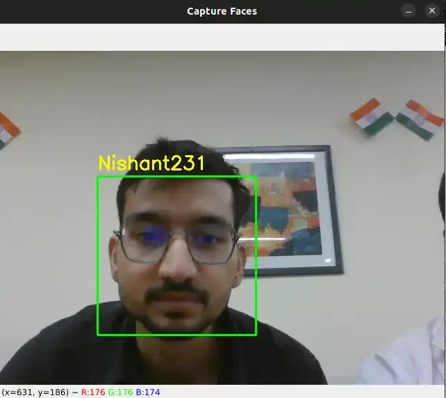
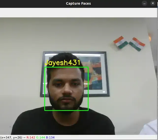
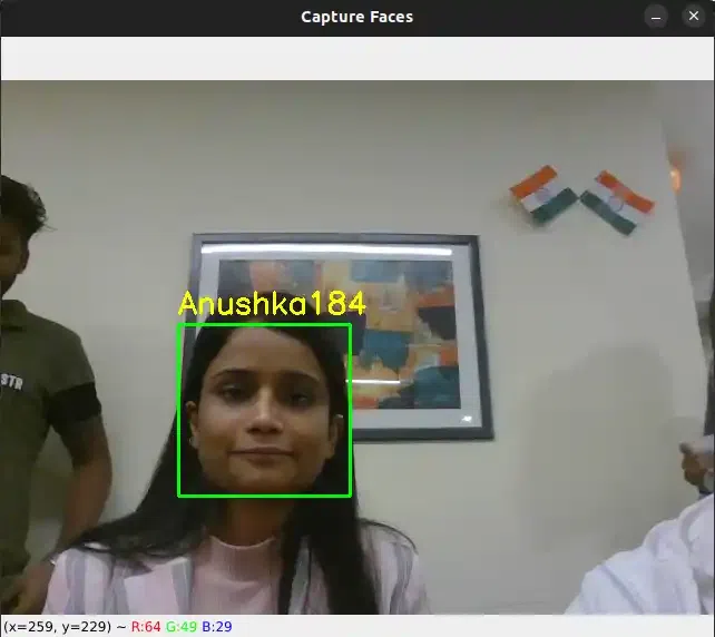
Next, we will run the capture_images() function, it will launch the camera and capture the images, then convert them into grayscale and save the images for further extraction of facial features and train the model. All the images are stored in the local dataset folder names ‘Faces’, to access it easily.

Capture the first Person Image

• Python3

# Create the dataset of faces

Output:

Capture the Second Person Image

• Python3

# Create the dataset of faces

Output:

Capture the Third Person Image

• Python3

capture_images('Anushka')

Output:

Similarly We can capture more persons images

capture_images('Shivang')
capture_images('Nishant')
capture_images('Laxmi')
capture_images('Jayesh')
capture_images('Abhishek')
capture_images('Suraj')

These all images are saved with their respective names

Create a dictionary of respective Usernames to encode into the numerical vector

• Python3

label = {'Shivang':0,'PawanKrGunjan':1,'VipulJhala':2,

Output:

{'Shivang': 0,
 'PawanKrGunjan': 1,
 'VipulJhala': 2,
 'Nishant': 3,
 'Laxmi': 4,
 'Jayesh': 5,
 'Abhishek': 6,
 'Anushka': 7,
 'Suraj': 8}

Step 4: Defining the Function to Train the Model

The code expects the existence of a correctly populated “Faces” directory containing grayscale face images labelled with the user number as part of the file name (e.g., “user1.jpg”, “user2.jpg”, etc.). Here we will train the LBPH face recognizer model i.e. recognizer using this dataset.

1. The function creates two empty lists, faces and labels, to store the face samples and labels, respectively. These lists will be used to collect the information needed to train the face recognition model.

2. The function iterates through the files in the “Faces” directory using a loop. It is assumed that the face images are saved in this directory as ‘.jpg’ files. The command os.listdir(‘Faces’) returns a list of filenames in the “Faces” directory.

3. Extract Label from File Name: The function extracts the label from the file name of each image file in the “Faces” directory. It assumes the file name format is “user_X.jpg,” where, ‘user’ is the name of the faces X represents the image’s counts to save the image.

4. Then we create a dictionary of name label which converts the user name string value into numericals values.

5. The function reads the image from the file path returned by os.path.join() using cv2.imread().

6. To detect faces in a grayscale image, use the face_cascade.detectMultiScale() method. This approach looks for faces at various scales in an image. The recognised faces are returned as a list of rectangles (x, y, width, height), which are saved in the face variable.

7. Before appending the face sample and label to the lists, the programme scans the image for any faces. This is accomplished by determining whether the length of the face variable is larger than zero, indicating that at least one face was spotted in the image.

8. If a face is discovered (len(face) > 0), the face sample is cropped from the grayscale image using information from the first entry of the face list (face[0]). The cropped face sample is added to the faces list, and the label associated with it is added to the labels list.

9. The function calls recognizer.train(faces, np.array(labels)) to train the face recognition model after iterating through all of the images in the “Faces” directory. The face samples are stored in the faces list, and the accompanying labels are stored as a NumPy array in np.array(labels).

Training

Next we split the dataset into training and testing subsets, it can be done by creating two lists named faces and labels for training the datasets. Then use the training subset to train a classifier on the extracted features. From the datasets, the model is trained to recognize the features.

• Python3

def train_model(label):

Output:

< cv2.face.LBPHFaceRecognizer 0x7fe13ef3bef0>

Step 5: Defining the Function to Recognize Faces

• cv2.VideoCapture(0) is used to launch the default camera (typically the primary webcam) for live video capture. The cap variable represents the video capture object.

• Reverse keys and values in the label dictionary to convert the numerical label to user name

• The function enters a loop that captures frames from the camera, analyses them, and recognises faces in real-time.

• Using cap.read(), the function reads a single frame from the camera within the loop. The return value ret shows if the frame was successfully read, and the frame data is kept in the frame variable.

• cv2.cvtColor(frame, cv2.COLOR_BGR2GRAY) is used to convert the frame to grayscale.

• The function detects faces in the grayscale frame using the previously developed face_cascade classifier. face_cascade.detectMultiScale() recognises faces at various scales in an image. The detected faces are returned as a list of rectangles (x, y, width, height), and this information is saved in the faces variable.

• The function uses the trained facial recognition model (recognizer) to predict the label and confidence level for each face sample. Using recognizer.predict(), we can get the predicted label and confidence on the cropped face region in the grayscale frame.

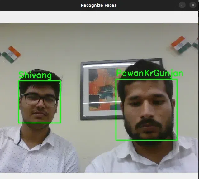
• The recognised face label is printed on the console. If the label is 0, it signifies the face is unrecognised or unknown. Otherwise, the recognised label (e.g., “1”, “2”, etc.) is printed. In addition, the recognised label and confidence level are displayed on the frame using cv2.putText() to demonstrate real-time recognition results.

• To highlight the recognised face, a green rectangle has been drawn around the identified face on the original colour frame using cv2.rectangle().

• Using cv2.imshow(), the frame with the face recognition results is displayed on the screen.

• The loop can be ended by pressing the ‘q’ key. The code uses cv2.waitKey(1) to wait for a short period of time (1 millisecond) before checking for the presence of the ‘q’ key (cv2.waitKey(1) & 0xFF == ord(‘q’)). If the ‘q’ key is pressed, the loop is broken, and the function continues to release the camera and dismiss all OpenCV windows.

• After breaking the loop, the code uses cap.release() and cv2.destroyAllWindows() to release the camera and close all OpenCV windows.

• Python3

# Function to recognize faces

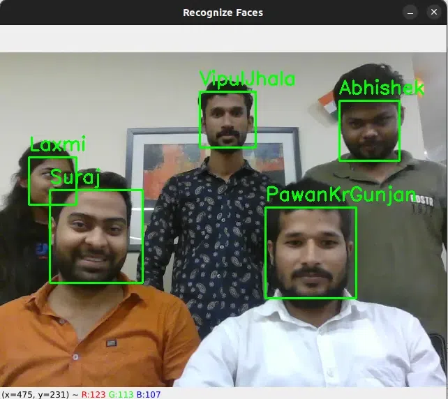
Feature Recognition:

Again we open the camera to capture an image, now it compares the detected grayscale frame with the trained model. If the face is not recognized (label equals 0) then the captured faces are not present in the label which we trained earlier. So this prints “Unknown Face”, else (label equals to a value) it recognized the face from the trained label and prints “Recognized Face: 1”. If we train the ‘n’ number of faces, then it stores it with label values 1,2,3., and so on.

• Python3

# Recognize the live faces

Output:

Conclusions

The Local Binary Patterns (LBPs) face recognizer model given in the code is a practical implementation for real-time face identification. It starts by capturing face images with the capture_images() function, allowing users to create a dataset with labelled faces. The train_model() function then extracts and trains facial features with the LBPs technique and OpenCV’s Haar Cascade Classifier. Following that, the recognize_faces() method employs the trained model to recognise faces in the webcam feed, providing real-time face labels and confidence ratings.