Step-by-Step Guide to Logistic Regression for Classification
 Vamshi A
What is Classification?
When it comes to Machine Learning, the 2 most commonly used algorithms are Linear and Logistic Regression. In this article I'm going to explain the second most commonly used machine learning algorithm - Logistic Regression.
In classification we try to identify our datapoints or objects as a part of a group. We are grouping data into different classes. For example, consider positive integers i.e, 1, 2, 3, ...etc. Here we can classify these numbers as even and odd numbers. If a number is divisible by 2 then it is even, odd otherwise. This grouping of data into different classes is called classification.
There are 2 types of classification:
Binary Classification
Multiple Classification
Binary Classification
Binary classification is exactly as it sounds. Binary means something involving just 2 things. In Binary Classification we try to classify our data points into 2 different classes, either "a" or "b". To explain it in mathematical terms, we classify our data as either 0 or 1.
Multiple Classification
Multiple classification refers to classifying our data into multiple categories or groups. In multiple classification we classify our data points into a category belonging to either 0 or 1 or 2 and so on.
Why not linear regression?
Some might argue that we can use linear regression for classification. But here's why linear regression is not a good fit for classification
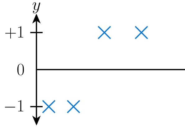
Linear regression works by fitting a straight line called the "Line of best fit" to the dataset given. This means that we use the line as a boundary to predict the output for our inputs. Let's assume our data points are given as below:

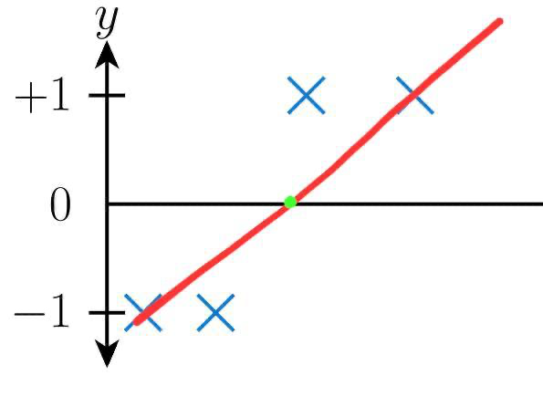
When we fit a line using linear regression for the following data, our line of best fits looks as follows:

This clearly shows that any data point left of the green point in the above picture is classified as -1 and any data points right side of the green point is classified as +1
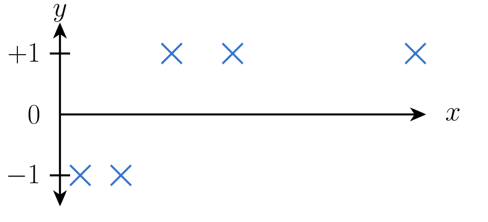
However, what if our data points are like this:

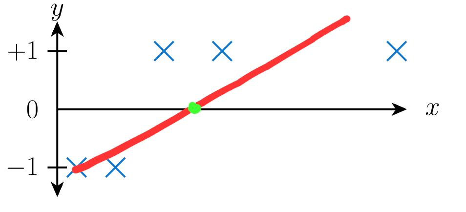
When we fit a straight line to the above picture, we might get the following:

This makes it obvious that not everything left of the green point from above picture should be labelled as -1, as there is a +1 present on the left side as well. So, linear regression is not recommended for classification problems.
Logistic Regression
We know that, for classification algorithms the output is either 0 or 1. So using linear regression which gives distinct values is an obvious no. Hence we use logistic regression.
So let's understand logistic regression. We know that the output we want is 0 or 1. This means that our hypothesis function h(θ) must give only either 0 or 1.
$$h_\theta (x) ∈ [0, 1]$$
Because of this condition we use a function called "Sigmoid function".
$$g(x) = \frac{1}{1 + \exp(-x)}$$
This means our hypothesis function is gonna be equal to:
$$\displaylines{ h_{\theta}(x) = g(\theta^Tx) = \frac{1}{1 + \exp(-\theta^Tx)} }$$
This is called the sigmoid or logistic function. The speciality of this function is that the value of this function lies only between 0 and 1. The graph plotted for this function looks as shown below:
Let's assume
$$\displaylines{ P( y = 1 | x ; \theta ) = h_\theta(x) \\ P(y = 0 | x ; \theta) = 1 - h_\theta(x) \\ }$$
This gives us the probability of y = 1 given x parameterised by θ equal to h(x) and, the probability of y = 0 given x and parameterised by θ equal to 1 - h(x). If we consider the fact that y only has values 0 or 1.
This gives us the following equation:
$$P(y | x; \theta) = h_\theta(x)^y (1 -h_\theta(x))^{1-y}$$
Taking the likelihood of the parameters theta gives us
$$\displaylines{ L(\theta) = P(\hat{y}|x^i;\theta) \\ = \prod_{i = 1}^mP(y^i|x^i;\theta) \\ \;\;\;\;\;\;\;\;\;\;\;\;\;\;\;\;\;= \prod_{i = 1}^m(h(x^i)^{y})(1 - h(x^i))^{1-y} }$$
Taking logarithm of the above equation
$$\displaylines{ l(\theta) = logL(\theta) \\ = \sum_{i = 1}^m y^i log(h_\theta(x)) + (1-y^i)log(1-h_{\theta}(x)) }$$
We need to choose a value of θ that maximises log likelihood of theta. To achieve this we use Batch Gradient Ascent:
$$\displaylines{\theta_{(j)} := \theta_j + \alpha\frac{\partial}{\partial\;\theta_j}l(\theta) \\ Let's \;\; do \;\; the \;\; partial \;\; derivation: \;\; \\ \frac{\partial}{\partial \;\theta_j}l(\theta) = \frac{\partial}{\partial \;\theta_j} \sum_{i = 1}^m y^i log(h_\theta(x)) + (1-y^i)log(1-h_{\theta}(x))\\ let's\;\; take\;\; out \;\; the \;\; sumation \;\; for \;\;now \\ = y^i\frac{\partial}{\partial \;\theta_j}log(h_\theta(x)) + (1-y^i) \frac{\partial}{\partial \;\theta_j}log(1-h_\theta(x)) \\ = y^i(\frac{1}{h_\theta(x)})\frac{\partial}{\partial \;\theta_j}(h_\theta(x)) +(1-y^i)\frac{1}{1-h_\theta(x)}\frac{\partial}{\partial \;\theta_j}(1 - h_\theta(x)) \\ = y^i(\frac{1}{h_\theta(x)})\frac{\partial}{\partial \;\theta_j}(h_\theta(x)) +(1-y^i)\frac{1}{1-h_\theta(x)}( 0 - \frac{\partial}{\partial \;\theta_j}(h_\theta(x))) \\ As \;\; the \;\; derivative \;\; of \;\; a \;\; constant \;\; is \;\; equal\;\; to\;\; 0 \\ = y^i(\frac{1}{h_\theta(x)})\frac{\partial}{\partial \;\theta_j}(h_\theta(x)) - (1-y^i)\frac{1}{1-h_\theta(x)}\frac{\partial}{\partial \;\theta_j}(h_\theta(x)) \\ = [ \;\; y^i(\frac{1}{h_\theta(x)}) - (1-y^i)\frac{1}{1-h_\theta(x)} \;\; ] \frac{\partial}{\partial \;\theta_j}(h_\theta(x)) \\ Now \;\; let's \;\; do \;\; the \;\; partial \;\; derivative \;\; of \;\; (h_\theta(x)) \\ }$$
Before we do the derivative of our hypothesis function, let's take a step back to consider our hypothesis function. As mentioned above our hypothesis function is equal to the sigmoid function. So let's do the derivative of the sigmoid function.
$$\displaylines{ We \;\; know \;\; that \;\; h_\theta(x) = g(\theta^Tx) = \frac{1}{1 + \exp^{-\theta^Tx}} \;\; which \;\; is \;\; a \;\; sigmoid \;\; function \\ \frac{\partial}{\partial \;\theta_j}(\frac{1}{1 + \exp(-\alpha)}) = \frac{\partial}{\partial \;\theta_j}(1 + \exp(-\alpha))^{-1} \\ = -(1 + \exp(-\alpha))^{-2} \frac{\partial}{\partial \; \theta_j}(\exp({-\alpha})) \\ = \frac{1}{(1 + \exp(-\alpha))^2}(\exp({-\alpha})) \\ = \frac{1}{1 + \exp(-\alpha)}\frac{\exp(-\alpha)}{1 + \exp(-\alpha)} \\ = \frac{1}{1 + \exp(-\alpha)}\frac{1 + \exp(-\alpha) - 1}{1 + \exp(-\alpha)} \\ Here, \;\; we \;\; add \;\; and \;\; subtract \;\; 1 \;\; on \;\; the \;\; top \\ Now, \;\; this \;\; is \;\; equal \;\; to \\ = \frac{1}{1 + \exp(-\alpha)}(\frac{1 + \exp(-\alpha)}{1 + \exp(-\alpha)} - \frac{1}{1 + \exp(-\alpha)}) \\ = \frac{1}{1 + \exp(-\alpha)}(1 - \frac{1}{1 + \exp(-\alpha)}) }$$
This is simply equal to the following
$$\frac{\partial}{\partial \; \theta_j}h_\theta(x) = \frac{1}{1 + \exp(-\theta^Tx)}(1 - \frac{1}{1 + \exp(-\theta^Tx)}) = h_\theta(x)(1 - h_\theta(x))$$
Substituting this to continue our above derivation gives us the following
$$\displaylines{ = [ \;\; y^i(\frac{1}{h_\theta(x)}) - (1-y^i)\frac{1}{1-h_\theta(x)} \;\; ] \frac{\partial}{\partial \;\theta_j}(h_\theta(x)) \\ = [ \;\; y^i(\frac{1}{h_\theta(x)}) - (1-y^i)\frac{1}{1-h_\theta(x)} \;\; ] (h_\theta(x)(1 - h_\theta(x)))\frac{\partial}{\partial \; \theta_j}(\theta^Tx) \\ = [\; y^i(1 - h_\theta(x)) - (1 - y^i) (h_\theta(x)) \;] x \\ Here, \frac{\partial}{\partial \; \theta_j}(\theta^Tx) \;\; is \;\; equal \;\; to \;\; x \;\; as everything \;\; else \;\; is \;\; a \;\; constant. \\ = (y^i - y^ih_\theta(x) - h_\theta(x) + y^ih_\theta(x) )x\\ = (y^i - y^ih_\theta(x) - h_\theta(x) + y^ih_\theta(x))x \\ = (y^i - h_\theta(x))x \\ Bringing \;\; back \;\; the \;\; \sum \;\; to \;\;the \;\;equation\;\; gives \;\; us \\ = \sum{(y^i - h_\theta(x^i))x^i} }$$
This gives us the equation for our gradient ascent which is now:
$$\displaylines{ \theta_j := \theta_j + \alpha\sum{(y^i - h_\theta(x))x} \\ Here \;\; \alpha \;\; is \;\; the \;\; learning \;\; rate }$$
If you read my previous blog on linear regression you might recognise the above equation. Yes, this is the same equation as the linear regression's gradient descent with a minus symbol. But don't be mistaken. Here's the catch, the hypothesis function in both of these algorithms is different.
In linear regression our hypothesis function was equal to
$$h_\theta(x) = \sum_{i=0}^n{\theta_ix_i} \;\; where \;\; x_0 = 1$$
and in our logistic regression the hypothesis function is equal to
$$h_\theta(x) = g(\theta^Tx) = \frac{1}{1 + \exp(-\theta^Tx)}$$
the sigmoid function or also known as logistic function.
Now, let's implement this in code
First, we'll import the necessary modules
import numpy as np
from sklearn.datasets import load_breast_cancer
Here we import numpy to hold and manipulate data or arrays of large size and we import the "load_breast_cancer" dataset from sklearn.datasets.
Now, we load the data and separate features (inputs) and labels (outputs)
data = load_breast_cancer()
X = data.data
Y = data.target
Now we have both X and Y data. But here's the problem, in the equation we have assumed that x₀ = 1. Before we do that let's actually analyse data.
For this we're going to import pandas to turn our data into a DataFrame for better visualisation
import pandas as pd
df = pd.DataFrame(X)
df
# This gives us the following output

Here, we can see that there's 569 rows and 30 cols now. We need to add a new col with value = 1 for every row to get our x₀ = 1 during calculation.
Now let's check our Y values
import pandas as pd
df = pd.DataFrame(Y)
df

Our Y has just labels of either 0 or 1. We don't have to change anything in our Y data.
Let's now change our X we need to add x₀ = 1 for every set of feature in the feature set, so for that we'll do the following
m, n = X.shape
new_X = np.ones(shape=(m,31))
for i in range(m):
    new_X[i] = np.append([1], X[i])
X = new_X
We first create an array of our all 1's in our required shape i.e, the rows and columns. Then we replace the values from our original data along with 1 in 0th place by using the np.append function and we update the X.
import pandas as pd
df = pd.DataFrame(X)
df

As you can see we've added a new column making the shape of our dataset into 569 rows and 31 cols. And the 0th column is all 1's as we needed it to be.
Now we're gonna initialise our theta values as all ones
theta = np.ones(shape=(X.shape[1],1))
That creates a numpy array of 31 rows and 1 column with all values = 1
Now that we're done with creating or preparing all the necessary data. We need to create our hypothesis function and gradient ascent function to complete our algorithm.
Our hypothesis function is nothing but a sigmoid function which takes continuous values and return a value between 0 and 1. We can create that function as per it's formula like this:
$$h_\theta(x) = g(\theta^Tx) = \frac{1}{1 + \exp{(-\theta^Tx)}}$$
def sigmoid(x):
    return (1 / (1 + np.exp(-x)))
We define a function that takes a value x as its parameter and returns the sigmoid value of it. Here, we use the "np.exp" function to get the exponential value.
Now we need to define the "GradientAscent" function to change our theta value. We use the following formula for our gradient ascent function
$$\displaylines{ \theta_j := \theta_j + \alpha\sum{(y^i - h_\theta(x))} \\ Here \;\; \alpha \;\; is \;\; the \;\; learning \;\; rate }$$
def GradientAscent(theta, X, y, alpha=0.001, epochs=300):
    for epoch in range(epochs):
        for j in range(len(theta)):
            error = 0
            for i in range(len(X)):
                h = X.dot(theta)
                error += (y[i][0] - sigmoid(h[i][0]))
            theta[j] += alpha * error
Now, lets try to walk through this code line by line:
We're going to receive the input, expected output, theta, alpha and epochs
Our alpha is also called the learning rate which we initialised to 0.001 at the beginning
Epochs is the number of times the algorithm is gonna repeat itself which we initialised to 300 at first.
Now, we're going to first run this algorithm "epoch" number of times i.e, 300 times in this case
For each epoch iteration we'll iterate over each theta
For each theta we calculate the error and update theta
We do that by first initialising error to 0 and adding all the differences of y - h(x) for every x
After this we update theta by adding error * alpha to our original theta.
Now, we've created our algorithm, we can now call the gradient ascent function and update the theta values
GradientAscent(theta, X, y)
Now before we calculate our algorithm's efficiency, we need to change something with our outputs. If the value from our sigmoid function is above 0.5 we classify it as 1 and 0 if otherwise. Now, we can get the results for the same input feature vector X.
h = X.dot(theta)
result = np.array([0 if sigmoid(i) <= 0.5 else 1 for i in h])
We first get all the h(x) values and send them into sigmoid function one by one and classify 0's and 1's and create a result algorithm.
Now, we can check the accuracy of our model by using an accuracy function. While writing this function is pretty easy, we're going to import it from sklearn
from sklearn.metrics import accuracy_score
accuracy_score(y, result)
This gave me an accuracy of 89%. Which isn't bad at all for a naive algorithm such as this. You can increase or decrease the alpha and epoch values for different results.
The total code of the logistic regression algorithm is below:
import pandas as pd
import numpy as np
from sklearn.datasets import load_breast_cancer
from sklearn.metrics import accuracy_score

def sigmoid(x):
    return (1 / (1 + np.exp(-x)))

def GradientAscent(theta, X, y, alpha=0.001, epochs=300):
    for epoch in range(epochs):
        for j in range(len(theta)):
            error = 0
            for i in range(len(X)):
                h = X.dot(theta)
                error += (y[i][0] - sigmoid(h[i][0]))
            theta[j] += alpha * error

data = load_breast_cancer()
X = data.data
Y = data.target
m, n = X.shape
new_X = np.ones(shape=(m,31))
for i in range(m):
    new_X[i] = np.append([1], X[i])
X = new_X
theta = np.ones(shape=(X.shape[1],1))
y = Y.reshape(-1,1)
GradientAscent(theta, X, y, 0.00075, 50)
h = X.dot(theta)
res = np.array([0 if sigmoid(i) <= 0.5 else 1 for i in h])
accuracy_score(y, res)
By changing the alpha to 0.00075 and epochs to 50, I got an accuracy score of 90%.
Congratulations on making it this far; we're all done.
If you enjoyed this article, please consider buying me a coffee.
Here are a few documentation links for the modules I used in this code:
Follow me on my socials and consider subscribing, as I'll be covering more Machine Learning algorithms "from scratch".
Subscribe to my newsletter
Read articles from Vamshi A directly inside your inbox. Subscribe to the newsletter, and don't miss out.
Written by

