Bias-Variance Trade-off

In machine learning, the bias-variance trade-off is a fundamental concept used to evaluate the performance of a model. It helps explain the sources of error in predictions. The total error (expected loss) of a model can be decomposed into three components:

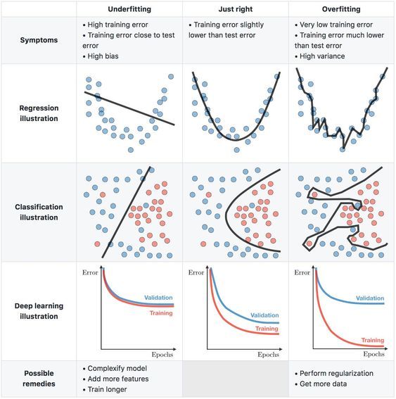
1. Bias: Error due to overly simplistic assumptions made by the model (e.g., underfitting).

2. Variance: Error due to sensitivity to small fluctuations in the training data (e.g., overfitting).

3. Irreducible error: Error inherent in the problem that cannot be reduced, often due to noise.

The expected error can be mathematically decomposed as follows:

Where:

Bias:

The bias measures the error due to the model's assumptions. It represents how much the average prediction differs from the true function. Mathematically:

• If the bias is high, the model is underfitting.

• Lower bias implies the model is making predictions closer to the true function.

Variance:

The variance measures the model's sensitivity to changes in the training dataset. It quantifies how much the model's predictions fluctuate when trained on different datasets. Variance is defined as the expected squared difference between a single prediction and the average prediction:

• High variance means the model's predictions vary a lot across different datasets (overfitting).

• Lower variance indicates more stable predictions across different datasets.

• 

  Bias tells us how closely our predictions are typically, or on average, aligned with the true value for the population or the actual outcome. In terms of the above bullseye diagram, how closely do our predictions on average land in the very centre of the bullseye?

  Variance tells us about the variability in our predictions. It tells us how tightly our individual predictions cluster. In other words, variance indicates how far and wide our predictions are spread. Do they span a small range or a large range?

• The data below (the red dots) comes from a randomly perturbed sine wave between 0 and ππ. I have three models that look at those red dots (the perturbed data) and try to predict the form or shape of the underlying curve:

  • a simple linear regression - which predicts a straight line

  • a quadratic regression - which predicts a parabola

  • a high-order polynomial regression - which can predict quite a complicated line

The linear regression (the straight blue line, top left) provides an under-fitted model for the curve evident in the data. The quadratic regression (the inverted parabola, bottom left) provides a reasonably good model. It is the closest of the models to a sine wave between the values of 0 and ππ. And the polynomial regression of degree 25 (the squiggly blue line, bottom right) over-fits the data and reflects some of the random noise introduced by the perturbation process.

• 

  The next chart compares the three blue models above, with the actual sine wave before the perturbation. The closer the blue line is to the red line, the less error the model has.

Coming back to the three-component cumulative error equation above, we can see the least total error occurs at an optimal point between a simple and complex model. Again, let's use a stylised chart to aid intuition.

As model complexity increases, the prediction error associated with bias decreases, but the prediction error from variance increases. This minimal total error sweet-spot (between simplicity and complexity) is the key insight of the bias-variance trade-off model. This is the best trade-off between the error from prediction bias and the error from prediction variance.