Understanding Quantization: Part I

Introduction

Quantization in general can be defined as mapping values from a large set of real numbers i.e., FP32 or even FP16 to values in a small discrete set most likely Int8 or Int4. There are recent works trying to map to 1bit models.

Typically it involves mapping continuous inputs to fixed values at the output. Usually Quantization in Digital Signal Processing can achieved in two ways

Rounding
Truncating

Rounding

Finding the nearest integer

$1.8 \rightarrow2\\$

$1.4 \rightarrow 1\\$

Truncating

Simply removing the least significant decimal part or entirely

$1.8 \rightarrow1\\$

$1.4 \rightarrow1\\$

Motivation

Mainly to improve the inference speed. Needless to say both the training and inference of the LLM are really costly. With the recent advent of really large language models, memory footprint is only getting higher and higher. Some common representation of model weights are

FP32
FP16
BF16
TF32
Int8

In general floating part numbers offer a broad range of values, consume less memory and enable the execution of complex computation with ease. They also tend to deliver faster performance and come in various formats making them ideal for a wide range of applications including gaming, simulations and machine learning.

How numbers are represented as floating points?

As you are aware, the floating point data type is widely used for its ability to represent a large range including fractional component. This makes it particularly useful in scenarios that require scientific notation. Such as scientific computations and precise data representations.

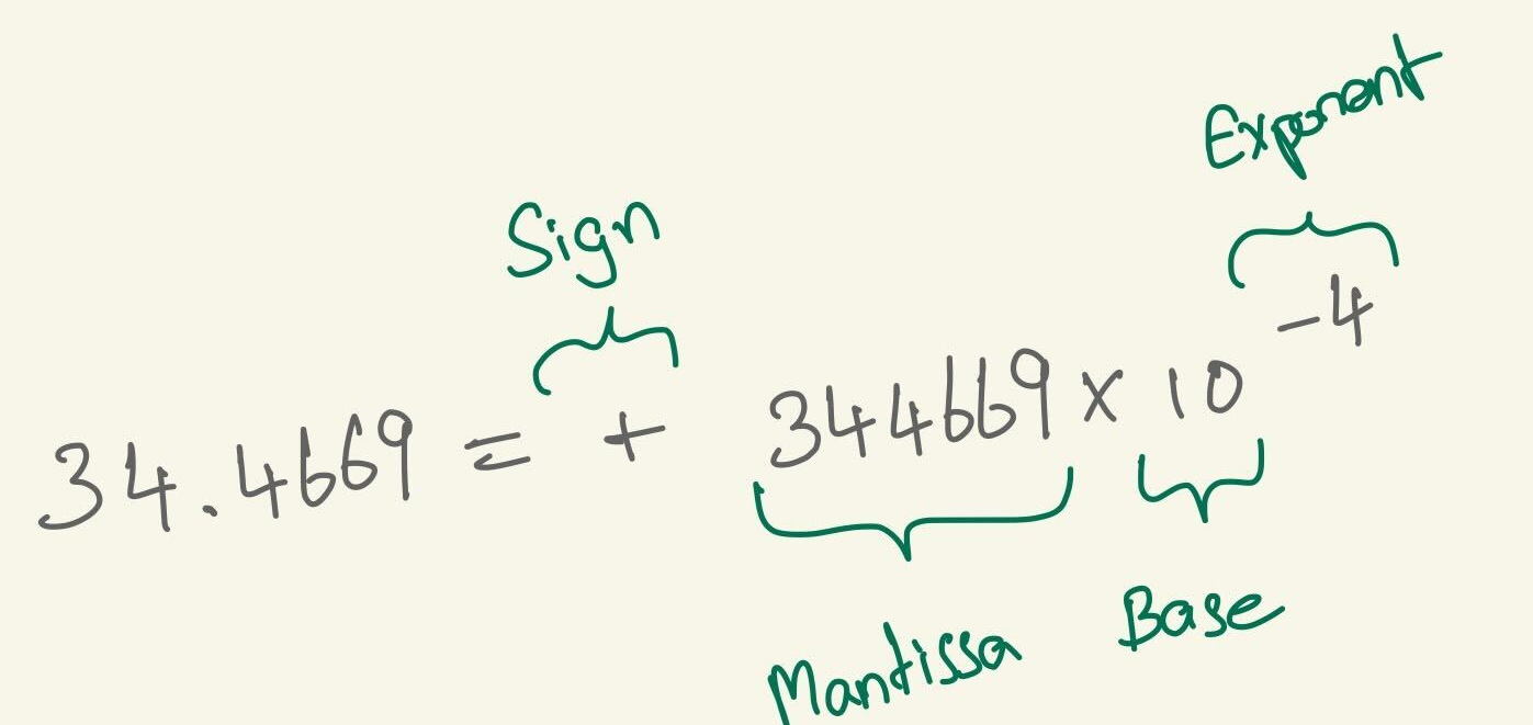
So this is how a floating point value of 34.4669 is represented under the hood. To break is down part by part

Sign : Whether the values is positive or negative.
Mantissa : Significand number.
Exponent : Integer value to use with the significand
Base : Base in which values are encoded.

Commonly used data types in Machine Learning

Floating point32 → Single/Full precision
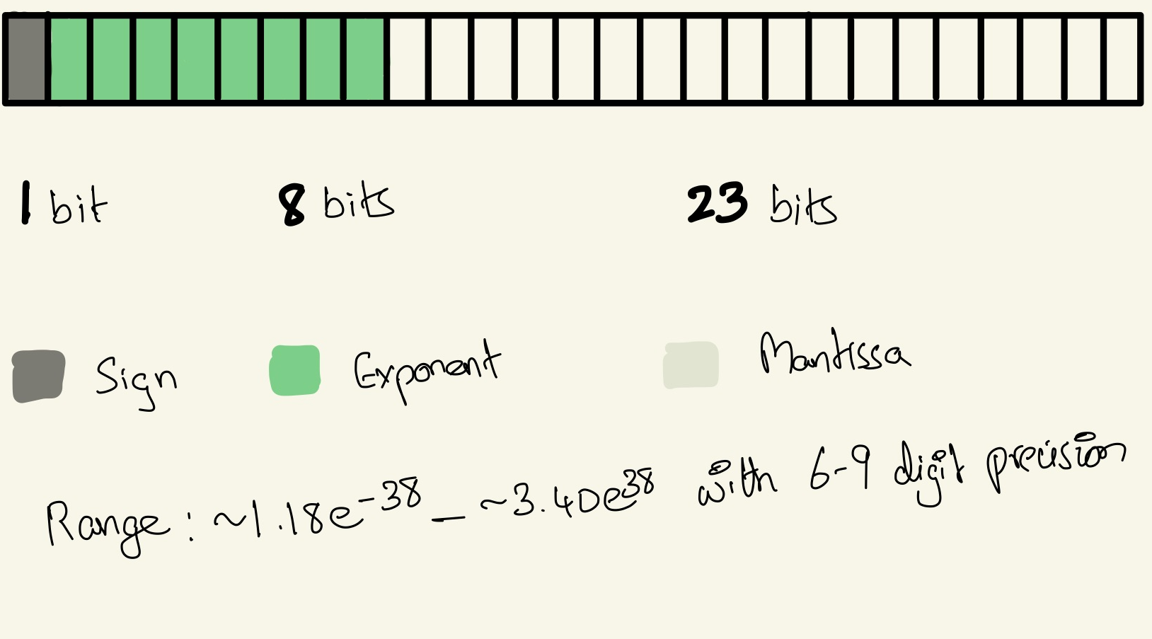
Floating point16 → Half precision
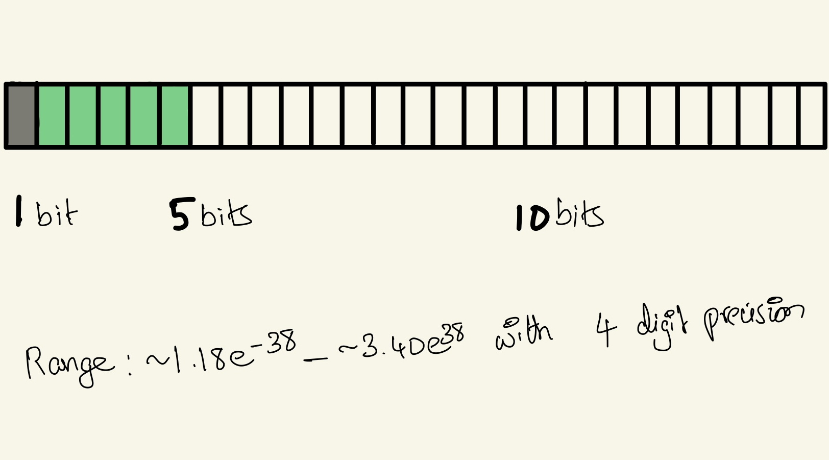
Brain Float16 → Half precision
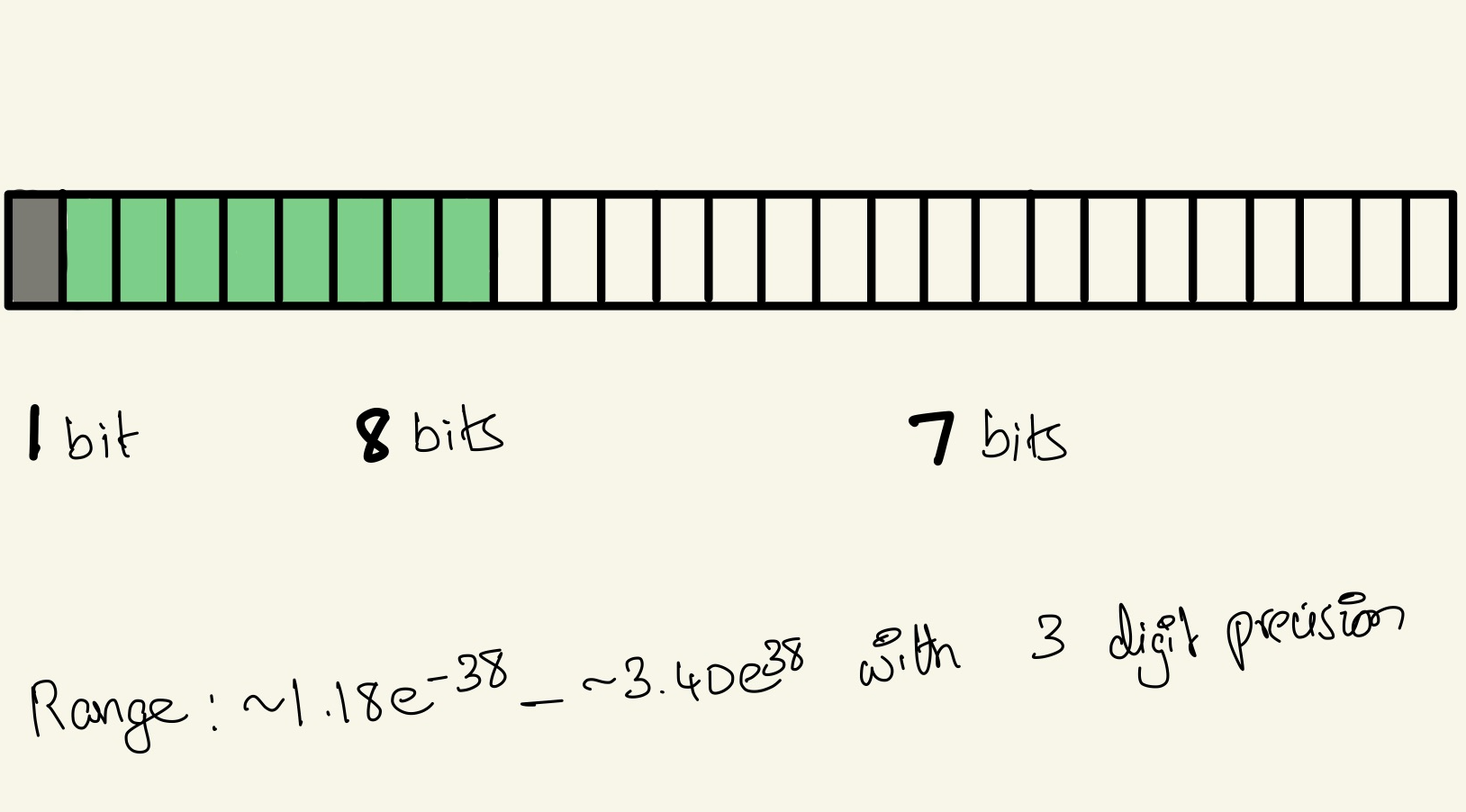
Tensor Float32

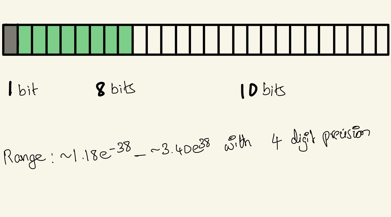
TF32 offers a significant advantage in the it requires minimal compiler support limited mainly to the bare bones level, particularly within the CUDA compiler. For the rest of the code-base, TF32 behaves similarly to FP32 maintaining the same dynamic range but with reduced precision. Leveraging TF32 is primarily about adjusting library calls to specify whether using TF32 is acceptable. It’s design allows for quick integration unlike BF16 and TF16 requiring more work since they involve different bit layouts, enabling developers to harness the performance benefits of Tensor cores with minimal effort.

Now that we have revised the floating point representation, we dive right back into Quantization.

In simple terms quantization is the conversion of weights from a higher memory format to a lower memory format. And there can two cases of quantization.

I) Uniform Quantization.

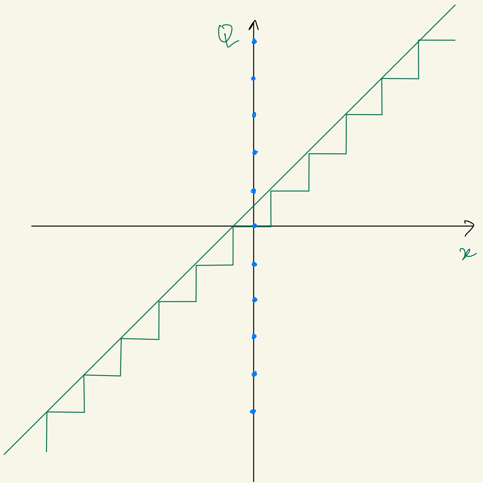
In the uniform quantization the conversation involves in mapping the input to be output in a linear function resulting in uniformly spaced outputs for uniformly spaced inputs.

II) Non-Uniform Quantization.

The mapping in this case is a non-linear function so the output wouldn’t be uniformly spaced for uniformly spaced inputs.

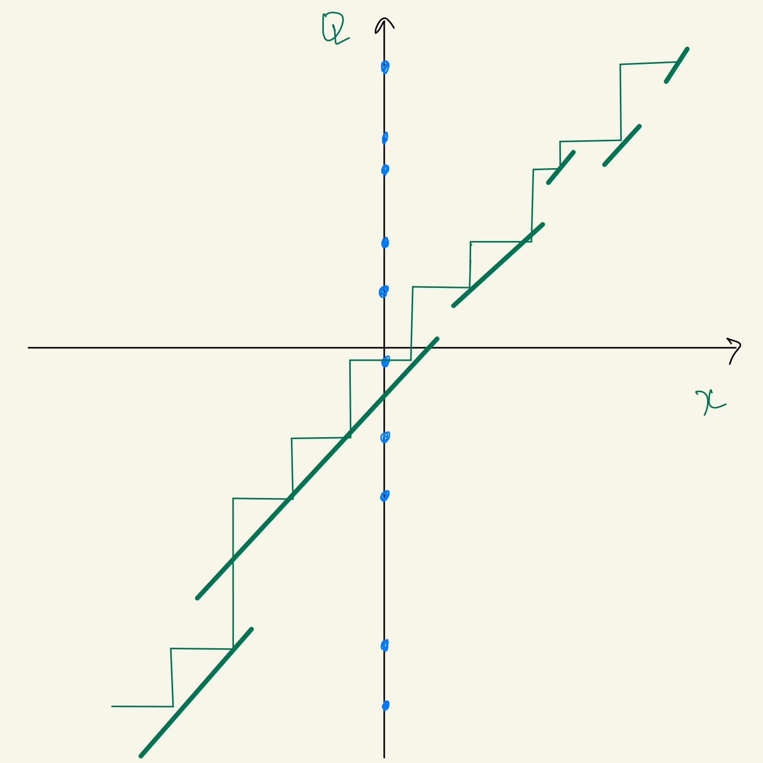
It’s quite easy to figure out the input representation values are not equally distributed so they are not equally represented on the output representation.

Uniform Quantization.

I) Symmetric Quantization

Most times in uniform quantization, the linear mapping function can be scaling, rounding or both.

$$\displaystyle \begin{array} \displaystyle Q = \displaystyle round(\frac{x}S) \\\\ \text{where:}\\ x = \text{Og floating point value}\\ S = \text{Scaling factor}\\ \end{array}$$

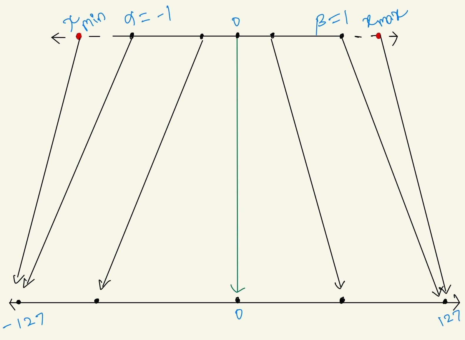
To transform the input representation to a light weight transformed representation, scaling factor $S\\$ is involved. This scaling factor helps in restricting the values of Float32 to Int8 within the ranges of $-127\\$ to $127\\$ and when the zero point of the input maps perfectly to be the zero point of the output then it is called Symmetric quantization.

II) Asymmetric Quantization

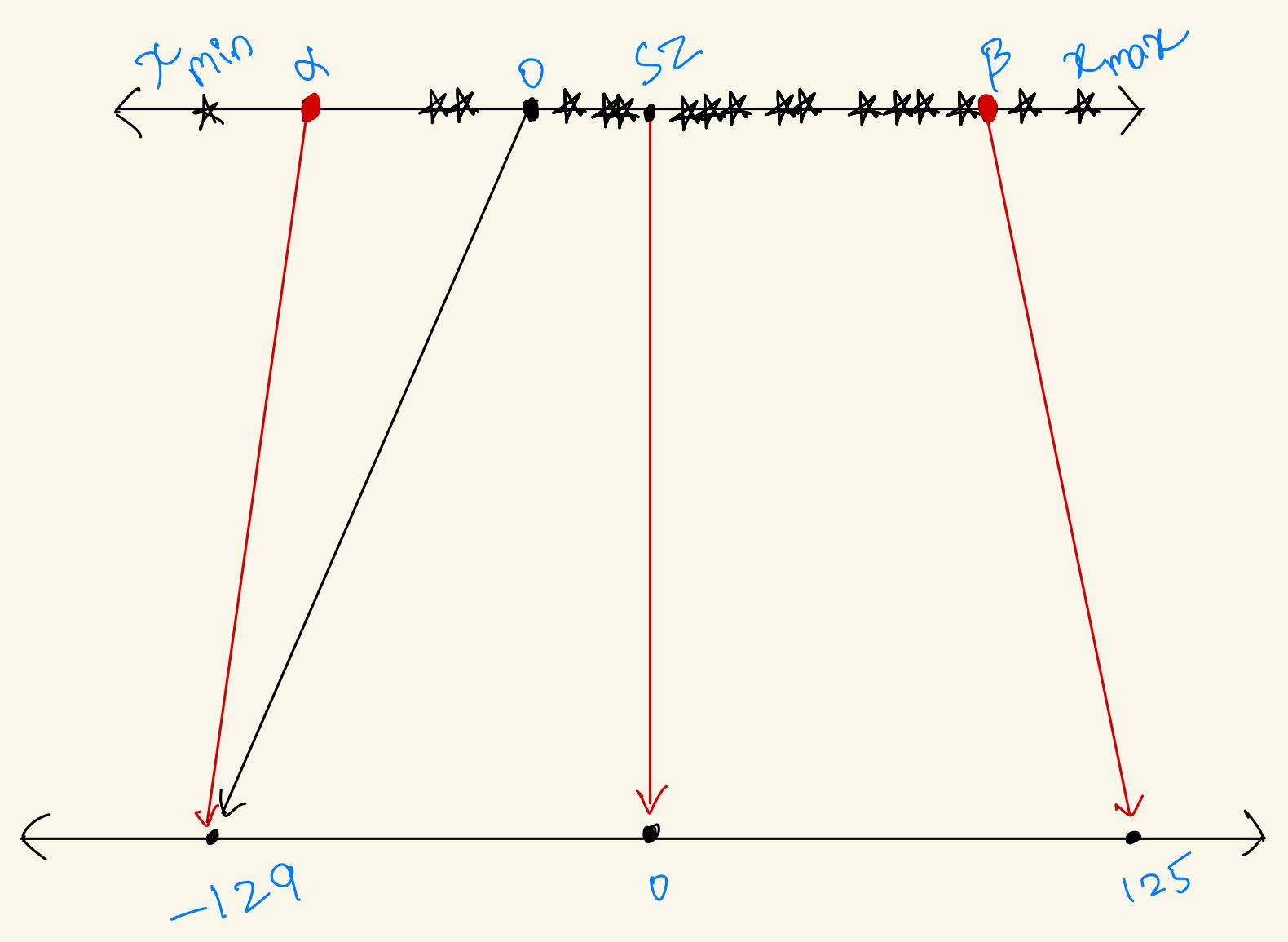
Now for a symmetric quantization the range of transformation should fall within $-127\\$ to $127\\$ to be able to transform the input values to an Int8 quantization. But if the range goes off rail say like $-129\\$ to $125\\$ which most times put off the input zero away from the output zero and this is called Asymmetric Quantization. Since the zero is off of its place we should count for it by adding a zero scale, now the equation becomes

$$\displaystyle \begin{array} \displaystyle Q = \displaystyle round(\frac{x}S) +Z \\\\ \text{where:}\\ Z = \text{Zero scale}\\ \end{array}$$

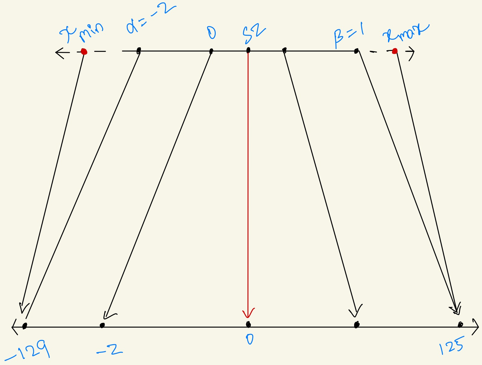
What is scaling and zero factor?

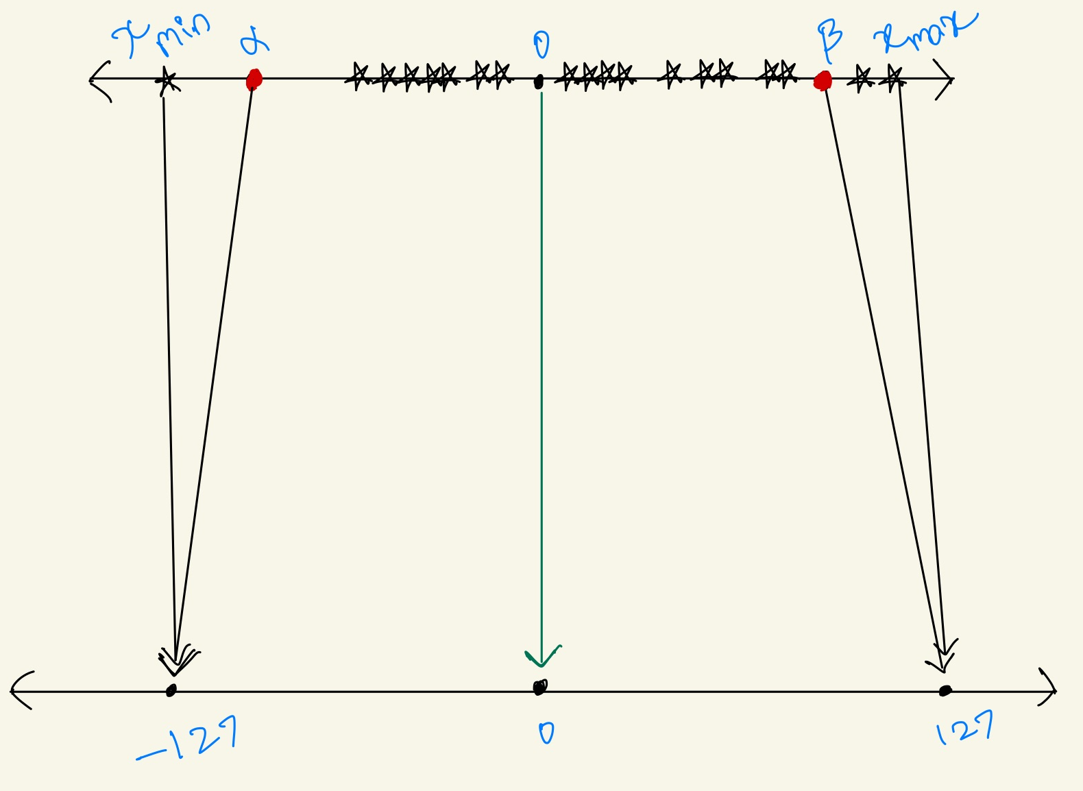
The scaling factor is a number which divides the entire range of numbers from the $\displaystyle x_{min}\\$ to $\displaystyle x_{max}\\$ across the input into uniform partition. We can choose to lip the input range beyond it’s max dense regions because anyway the values beyond the $\displaystyle x_{min}\\$ and $\displaystyle x_{max}\\$ would just fall onto the min and max of the output range i.e., here the minimum is $-127\\$ and maximum $127\\$. Now the process of choosing $\alpha$ and $\beta$ which helps in finding the clipping range is called Calibration.

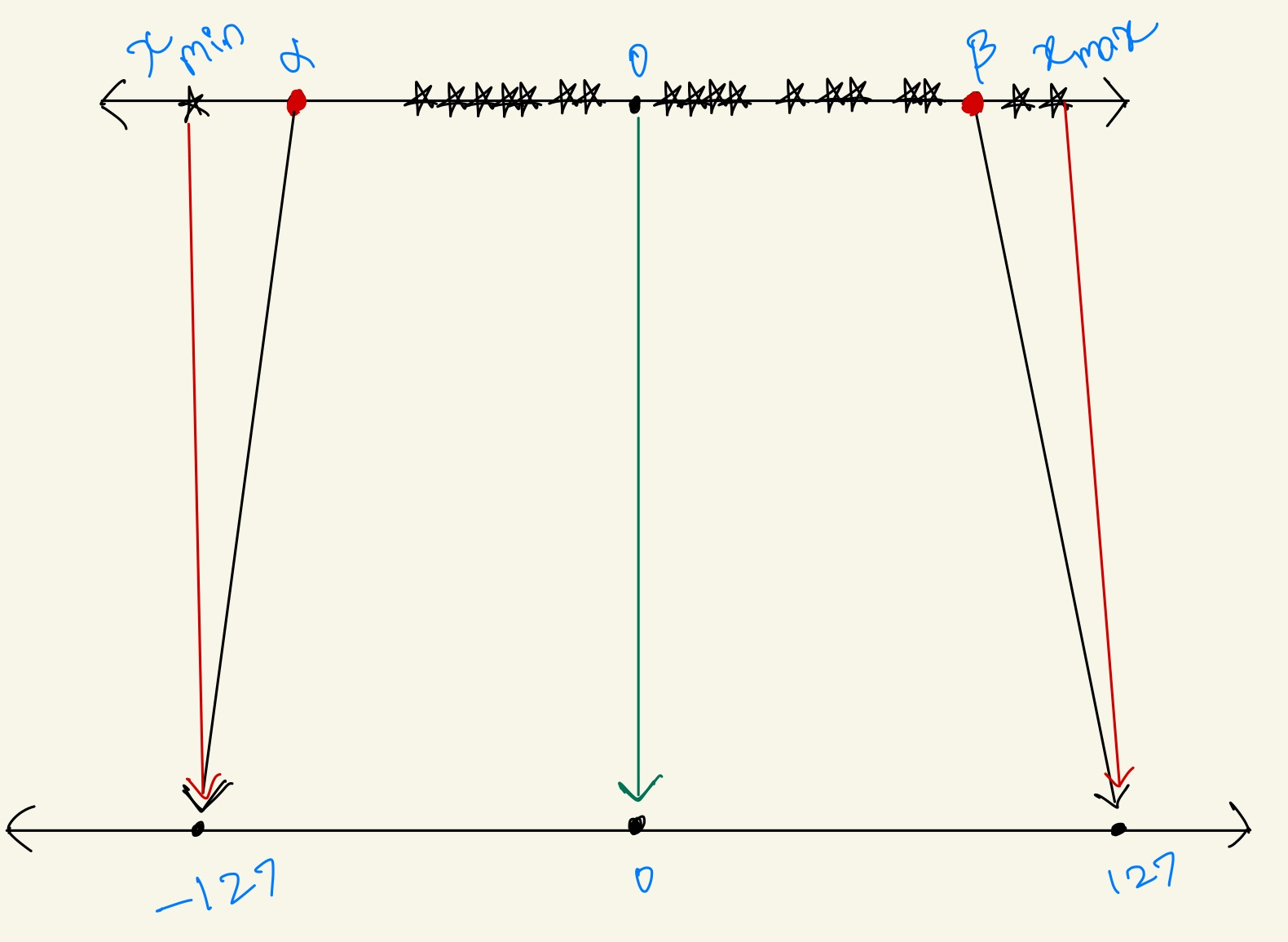
To avoid excessive clipping we can use this formula for

$$\begin{array}{llll} \displaystyle S = \displaystyle \frac{\beta-\alpha}{2^b-1} = \displaystyle \frac{x_{max}-x_{min}}{2^b-1} \\\\ \text{where:}\\ \alpha = x_{min}\\ \beta = x_{max}\\ b = \text{quantization bit width} \end{array}$$

Sometime the $\displaystyle x_{min}\\$ and $\displaystyle x_{max}\\$ values could be different and end up in an asymmetric manner. Ex: $\displaystyle x_{min}\\$ = -2.0 and $\displaystyle x_{max}\\$ = 1.0. So to constraint it to be a symmetric quantization,

$$\begin{array}{llll} \displaystyle -\alpha = \displaystyle \beta = \displaystyle max(|r_{min}|, |r_{max}|) \\ \displaystyle Z = \displaystyle 0 \\ \end{array}$$

ReLU and GeLU are most common examples for an asymmetric quantization. Why because the values are skewed on to one side i.e., these activation are only positive. It is also to consider the activation charges with each varying inputs.

De-quantization

One cool thing about quantization is one can always get back to its original representation $\bar{x}\\$ (i.e.,) the original floating point representation.

$$\begin{array}{llll} \displaystyle \bar{x}= \displaystyle S(Q+Z) \\ \displaystyle \bar{x}= \displaystyle r+e \\ i.e.\ \displaystyle x \neq \displaystyle \bar{x}\\ \end{array}$$

Here $\bar{x}\\$ is just an approximation of the original data point $x\\$. Usually in machine learning until the error is huge enough to hurt the accuracy and perplexity we don’t really bother about the output representation $\bar{x}\\$ being deviated from the original input representation $x\\$.

Types of Quantization

Post Training Quantization
Quantization Aware Training

Post Training Quantization

We start with the existing pre-trained model however we wouldn’t train it but calculate the calibration data which we use it to find the clipping range, scaling factor and zero factor. We get these values from the model values.

Quantization Aware Training

This is a tricky quantization technique because to be able to train a model it should be differentiable in the first place. But the quantization operation in non-differentiable to circumvent this issue, fake quantizers like Straight Through Estimator is used. During fine-tuning both the forward and backward of the quantized model use floating point values but then these parameters are quantized after each gradient update.

QAT helps in recovering the lost accuracy while training or any other metric. Although they provide good accuracy when compared over PTQ, however one downside is QAT needs more data to get the desirable results.

References:

A Survey of Quantization Methods for Efficient Neural Network Inference