Mathematical Transformers

When dealing with data, transforming columns using mathematical functions can significantly improve the performance of machine learning models. By applying various transformations, we can adjust the probability density function of our data to approximate a normal distribution, which is crucial for many statistical methods and models.

Mathematical transformations can be categorized into several types:

1. Logarithmic Transformations: This includes log, reciprocal, and square root transformations. These methods help manage skewed data by compressing the range of values and reducing the impact of extreme values.

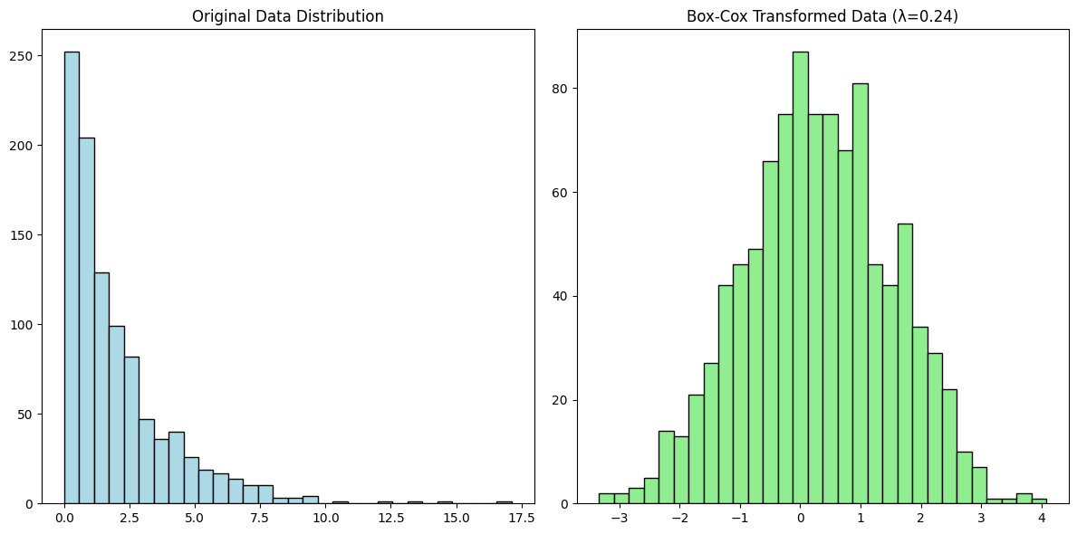
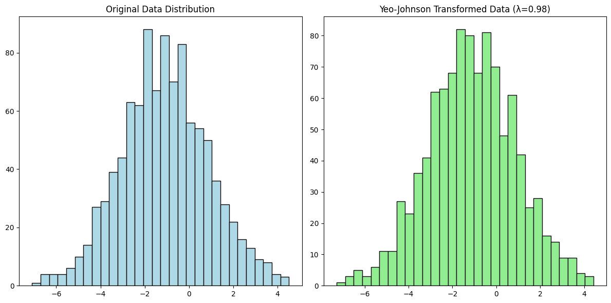
2. Power Transformations: The Box-Cox and Yeo-Johnson transformations fall into this category. These methods are designed to stabilize variance and make the data more normal. Box-Cox is suitable for positive data, while Yeo-Johnson can handle both positive and negative values.

Scikit-Learn Transformers

In scikit-learn, a powerful Python library for machine learning, we have several transformers to aid in these transformations:

• Function Transformer: This allows for custom transformations, including log, reciprocal, square root, and other user-defined functions.

• Power Transformer: Implements both Box-Cox and Yeo-Johnson transformations to normalize data.

• Quantile Transformer: Converts features to follow a uniform or normal distribution by ranking and scaling data.

Assessing Normal Distribution

To verify if the data follows a normal distribution, consider these methods to check so:

• Seaborn Displot: This visualization tool helps check data skewness by plotting the distribution of data. A normal distribution will appear bell-shaped.

• Skewness Metric: Using pd.skew() from pandas, we can quantify the skewness of our data. Values close to zero indicate a more normal distribution.

• QQ Plot: This scatter plot compares the quantiles of the data against the quantiles of a normal distribution. A straight line suggests that data is normally distributed.

By utilizing these transformations and evaluation techniques, we can better prepare your data for analysis and know if we even need to apply what we will learn about transformers.

Log Transform

The log transformation involves applying the logarithm function to each value in the dataset. Mathematically, it's expressed as:

y′=log⁡(x)

where x is the original value, and y′ is the transformed value.

import numpy as np
import pandas as pd
import seaborn as sns
import matplotlib.pyplot as plt


ages = np.random.randint(20, 61, size=1000)  #Ages between 20 and 60
weights = np.random.lognormal(mean=4, sigma=0.5, size=1000)  #Log distribution forright skew


data = pd.DataFrame({
    'Age': ages,
    'Weight': weights
})


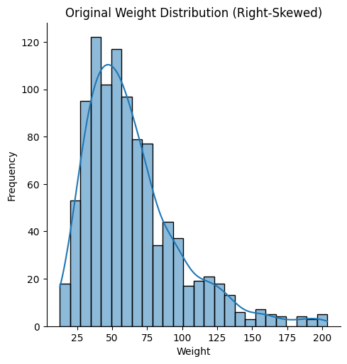
sns.displot(data['Weight'], kde=True)
plt.title('Original Weight Distribution (Right-Skewed)')
plt.xlabel('Weight')
plt.ylabel('Frequency')
plt.show()

#Applying log transformation
data['Log_Weight'] = np.log(data['Weight'])

#Plotting the normalized distribution
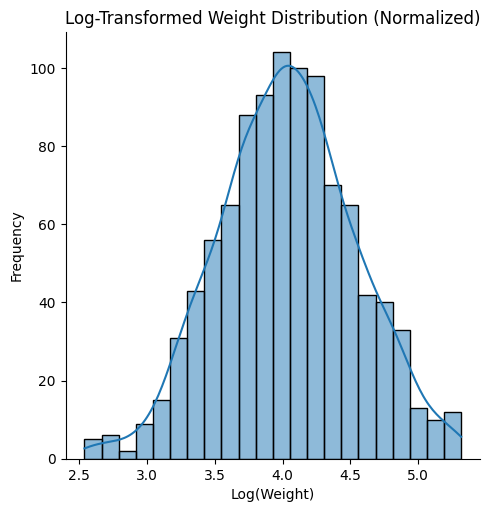
sns.displot(data['Log_Weight'], kde=True)
plt.title('Log-Transformed Weight Distribution (Normalized)')
plt.xlabel('Log(Weight)')
plt.ylabel('Frequency')
plt.show()

Applications and Benefits:

• Normalization: This transformation is particularly useful for right-skewed data, where there are a few extremely large values that can distort the overall distribution. By applying the log function, large values are compressed, making the data more normally distributed.

• Additive to Multiplicative: Log transformation changes the additive scale of data to a multiplicative scale. This means that rather than adding values together, the effect of each value is multiplied. For instance, in a log-transformed dataset, a change from 10 to 20 is equivalent to a change from 100 to 200, indicating a proportional change rather than an absolute one.

• This method is not suitable for negative values or zero, as the logarithm of these numbers is undefined.

• Often used in financial data to stabilize variance and in cases where data spans several orders of magnitude, such as income levels or stock prices.

Square Transform x^2

The Square Transformation involves squaring each value in the dataset:

y′=x^2

Applications and Benefits:

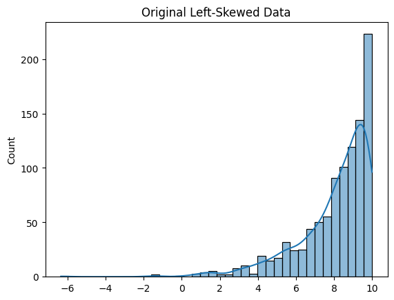
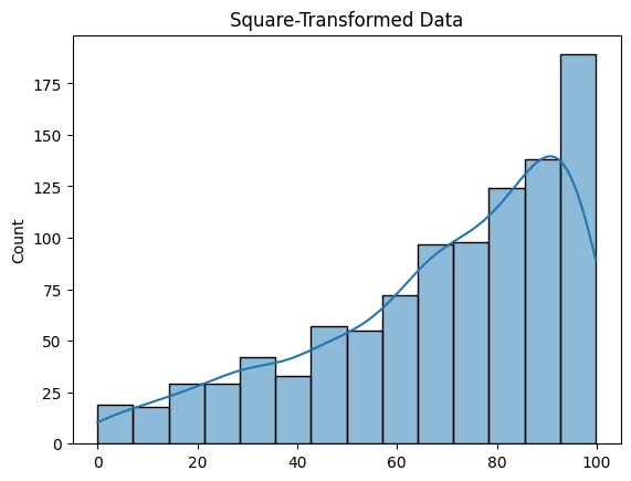
• Left-Skewed Data: This transformation is effective for left-skewed data, where the distribution has a long tail on the left. By squaring the values, you amplify the effect of larger values and reduce the skewness.

• Variance Increase: Squaring increases the variance, which can be useful if the dataset's variance is too low and needs adjustment.

• Impact on Normality: While this transformation can correct left skewness, it might not always lead to a normal distribution and can sometimes exacerbate the skewness if applied indiscriminately.

• Often used in quadratic regression models or scenarios where the relationship between variables is not linear but follows a parabolic trend.

import numpy as np
import matplotlib.pyplot as plt
import seaborn as sns
from scipy.stats import skew


np.random.seed(42)
left_skewed_data = np.random.exponential(scale=2, size=1000) * -1 + 10

#Plot the original left-skewed data
sns.histplot(left_skewed_data, kde=True)
plt.title('Original Left-Skewed Data')
plt.show()

#Square transformation
square_transformed_data = np.square(left_skewed_data)


sns.histplot(square_transformed_data, kde=True)
plt.title('Square-Transformed Data')
plt.show()
original_skewness = skew(left_skewed_data)
transformed_skewness = skew(square_transformed_data)

print(f'Original Skewness: {original_skewness}')
print(f'Square Transformed Skewness: {transformed_skewness}')

Reciprocal Transformation

Reciprocal transformation is useful when the data is highly skewed, and you want to reduce its skewness. This transformation involves taking the reciprocal (1/x) of each value in the dataset. It's particularly useful for dealing with long-tailed distributions, as it compresses large values more than small ones.

Let's say we have a dataset with highly skewed continuous variables, like house prices or transaction amounts. A reciprocal transformation can make the data more normally distributed, which is beneficial for many machine learning models, particularly linear models that assume normality.

Applications and Benefits:

• Scale Adjustment: This transformation is effective in managing large values by converting them into smaller ones, and vice versa. It also helps in reducing the influence of outliers.

• Impact on Skew: Reciprocal transformation can be particularly useful for data with a strong right skew, as it inversely adjusts the values, thus flattening the distribution.

• Handling Zeros: This method does not handle zero values well because the reciprocal of zero is undefined. Care must be taken to address zero values before applying this transformation.

• Useful in scenarios where the range of values is very large and where you need to reduce the impact of extreme values, such as in data from scientific measurements.

Box Cox Transform

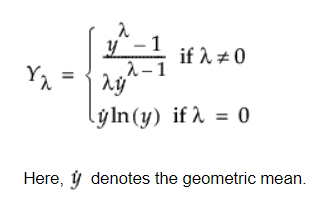
The optimal value of λ is typically determined through maximum likelihood estimation or by cross-validation. The goal is to find a λ that makes the transformed data as close to normally distributed as possible. Lambda usually varies from -5 to 5.

import numpy as np
import pandas as pd
import matplotlib.pyplot as plt
from scipy.stats import boxcox
from scipy.stats import norm


np.random.seed(0)
data = np.random.exponential(scale=2, size=1000)

#Plotting the original data distribution 
plt.figure(figsize=(12, 6))
plt.subplot(1, 2, 1)
plt.hist(data, bins=30, color='lightblue', edgecolor='black')
plt.title('Original Data Distribution')

#Applying Box-Cox transformation and plotting 
transformed_data, best_lambda = boxcox(data)
plt.subplot(1, 2, 2)
plt.hist(transformed_data, bins=30, color='lightgreen', edgecolor='black')
plt.title(f'Box-Cox Transformed Data (λ={best_lambda:.2f})')

plt.tight_layout()
plt.show()

Yeo Johnson Transform

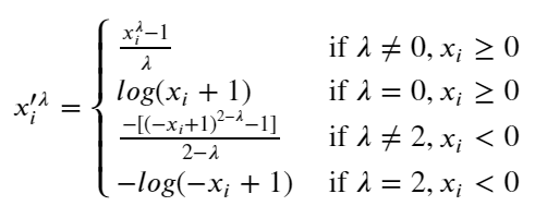
The Yeo-Johnson Transformation is an extension of the Box-Cox transformation designed to handle both positive and negative values in a dataset. It is particularly useful when dealing with data that includes zero or negative values, which cannot be transformed using the Box-Cox method.

import numpy as np
import pandas as pd
import matplotlib.pyplot as plt
from scipy.stats import yeojohnson
np.random.seed(0)
data = np.random.randn(1000) * 2 - 1 

plt.figure(figsize=(12, 6))
plt.subplot(1, 2, 1)
plt.hist(data, bins=30, color='lightblue', edgecolor='black')
plt.title('Original Data Distribution')

#Applying yeo johnson transformation
transformed_data, best_lambda = yeojohnson(data)
plt.subplot(1, 2, 2)
plt.hist(transformed_data, bins=30, color='lightgreen', edgecolor='black')
plt.title(f'Yeo-Johnson Transformed Data (λ={best_lambda:.2f})')

plt.tight_layout()
plt.show()

The transformer architecture represents a pivotal innovation in machine learning, effectively transforming the way we approach sequence transduction tasks such as language modelling and machine translation.

This architecture has proven its efficacy in various domains, establishing new benchmarks for translation tasks, as evidenced by achieving state-of-the-art BLEU scores in English-German and English-French translations​. The scalability of transformers, combined with their ability to be trained faster than previous models, has contributed to their widespread adoption in both academic research and industry.

As the machine learning community continues to refine the architecture with innovations like sparse transformers and more efficient attention mechanisms, the transformer’s ability to push the boundaries of what’s possible in AI will only grow stronger.

Read:

https://proceedings.neurips.cc/paper_files/paper/2017/file/3f5ee243547dee91fbd053c1c4a845aa-Paper.pdf