Introduction to Spark Optimization

Optimizing Spark can dramatically improve performance and reduce resource consumption. Typically, optimization in Spark can be approached from three distinct levels: cluster level, code level, and CPU/memory level. Each level addresses different aspects of Spark's operation and contributes uniquely to overall efficiency in distributed processing with Spark.

Cluster Level Optimization

At the cluster level, optimization involves configuring the Spark environment to efficiently manage and utilize the hardware resources available across the cluster. This includes tuning resource allocation settings such as executor memory, core counts, and maximizing data locality to reduce network overhead. Effective cluster management ensures that Spark jobs are allocated the right amount of resources, balancing between under-utilization and over-subscription.

Code Level Optimization

Code level optimization refers to the improvement of the actual Spark code. It involves refining the data processing operations to make better use of Spark’s execution engine. This includes optimizing the way data transformations and actions are structured, minimizing shuffling of data across the cluster, and employing Spark's Catalyst optimizer to enhance SQL query performance. Writing efficient Spark code not only speeds up processing times but also reduces the computational overhead on the cluster.

CPU/Memory Level Optimization

At the CPU/memory level, the focus shifts to the internals of how Spark jobs are executed on each node. This entails tuning garbage collection processes, managing serialization and deserialization of data, and optimizing memory usage patterns to prevent spilling and excessive garbage collection. These optimizations, utilizing the Tungsten optimizer, enhance the utilization of available CPU and memory resources, which is essential for efficiently processing large-scale data.

In this article, we will mostly be diving into code level optimisation based on the code we worked with in the previous articles.

Narrow and Wide Transformations

Narrow Transformations

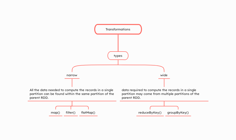
Narrow transformations involve operations where data required to compute the elements of the resulting RDD can be derived from a single partition of the parent RDD. This means there is no need for data to be shuffled across partitions or across nodes in the cluster. Each partition of the parent RDD contributes to only one partition of the child RDD.

Examples of Narrow Transformations:

• map(): Applies a function to each element in the RDD.

• filter(): Returns a new RDD containing only the elements that satisfy a predicate.

• flatMap(): Similar to map, but each input item can be mapped to zero or more output items.

Because data does not need to move between partitions, narrow transformations are generally more efficient and faster.

Wide Transformations

Wide transformations, also known as shuffle transformations, involve operations where data needs to be shuffled across partitions or even across different nodes. This happens because the data required to compute the elements in a single partition of the resulting RDD may reside in many partitions of the parent RDD.

Examples of Wide Transformations:

• groupBy(): Groups data according to a specified key.

• reduceByKey(): Merges the values for each key using an associative reduce function.

• join(): Joins different RDDs based on their keys.

Wide transformations are costlier than narrow transformations because they involve shuffling data, which is an expensive operation in terms of network and disk I/O.

Spark Computation

When you write and run Spark code, how does it execute from start to finish to produce the output?

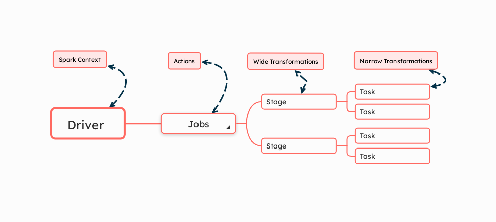
• Number of Jobs: In Spark, a job is triggered by an action. Each action triggers the creation of a job, which orchestrates the execution of stages needed to return the results of the action.

  Number of jobs = Number of actions

• Number of Stages: Stages in Spark are sets of tasks that are executed together on the same cluster node and can run in parallel. Stages are divided by wide transformations.

  Number of stages = Number of wide transformations + 1

• This +1 accounts for the final stage that gathers results following any necessary shuffles.

• Number of Tasks: Tasks are the smallest units of work in Spark and correspond to individual operations that can be performed on data partitions in parallel. The number of tasks is directly proportional to the number of partitions of the RDD (Resilient Distributed Dataset). A single task is spawned for each partition for every stage. Therefore, adjusting the number of partitions can significantly affect parallelism and performance.

  Number of tasks = Number of partitions

Catalyst Optimiser - The Internals

Unresolved Logical Plan

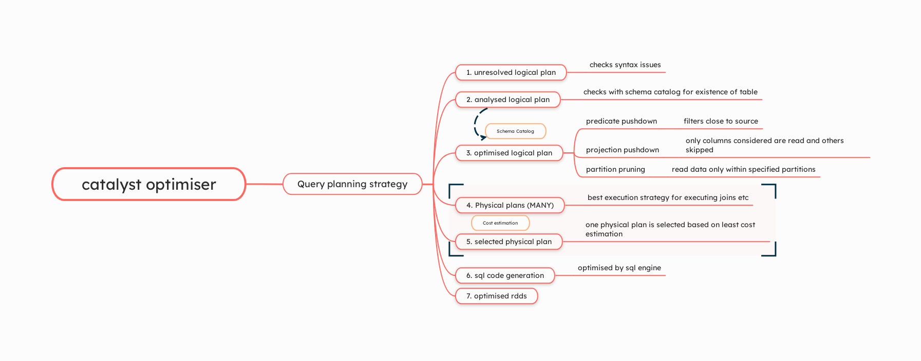
This is the initial plan generated directly from the user's query, representing the operations required without detailed knowledge of the actual data types and structure. If there are syntax-level issues such as missing brackets, incorrect function names, or syntactical errors, this plan will generate errors because it can't correctly interpret the query.

Analyzed Logical Plan

After the initial parsing, the query's logical plan is analyzed. This step involves resolving column and table names against the existing schema catalog. It checks whether the columns, tables, and functions referenced in the query actually exist and are accessible. If there are errors in the names or if referenced tables or columns don't exist, the query will fail at this stage.

Optimized Logical Plan - Rule-Based Optimization

Once the logical plan is analyzed and validated, it undergoes rule-based optimizations. These optimizations aim to simplify the query and improve execution efficiency:

• Predicate Pushdown

  Filters are applied as early as possible to reduce the amount of data processed in subsequent steps.

• Projection Pushdown

  Only necessary columns are retrieved, skipping over unneeded data, which minimizes I/O.

• Partition Pruning

  Reduces the number of partitions to scan by excluding those that do not meet the query's filter criteria.

Physical Plan

The optimized logical plan is then converted into one or more physical plans. These plans outline specific strategies for executing the query, including how joins, sorts, and aggregations are to be physically implemented on the cluster. The Catalyst Optimizer evaluates various strategies to find the most efficient one based on the actual data layout and distribution.

Cost Model Evaluation

From the possible physical plans, the Catalyst Optimizer uses a cost model to determine the best execution strategy. This model considers:

• Data distribution

• Disk I/O

• Network latency

• CPU usage

• Memory consumption

The optimizer assesses each plan's cost based on these factors and selects the one with the lowest estimated cost for execution.

Code Generation

This final step involves generating optimized bytecode or SQL code that can be executed by Spark's engine. The code is specifically tailored to be efficient based on the physical plan and the underlying execution environment (like JVM bytecode for operations on RDDs). The SQL code is further optimised by the SQL engine.

Execution of Optimized RDDs

The generated code leads to the execution of the plan on Spark's distributed infrastructure, creating optimized RDDs that carry out the intended data transformations and actions as defined by the query.

Caching

Cache and persist are mechanisms for optimizing data processing by storing intermediate results that can be reused in subsequent stages of data transformations. Here's a concise explanation of both:

Cache

• cache() in Spark stores the RDD, DataFrame, or Dataset in memory (default storage level), making it quickly accessible, speeding up future actions that reuse this data.

• The data is stored as deserialized objects in the JVM memory. This means the objects are ready for computation but occupy more space compared to serialized data.

Persist

• persist() method allows you to specify different storage levels, offering more flexibility compared to cache().

• You can choose how Spark stores the data, whether in memory only, disk only, memory and disk, and more. The choice affects the performance and efficiency of data retrieval and processing.

  • MEMORY_ONLY

    Default for persist(), similar to cache(), stores data as deserialized objects in memory.

  • DISK_ONLY

    Useful for very large datasets that do not fit into memory. It avoids the overhead of recomputing the data by storing it directly on the disk.

  • MEMORY_AND_DISK

    Stores partitions in memory, but if the memory is insufficient, it spills them to disk. This can help handle larger datasets than memory can accommodate without re-computation.

  • OFF_HEAP

    Available only in Java and Scala, this option stores data outside of the JVM heap using serialized objects. This is useful for managing memory more efficiently, especially with large heaps. We’ll discuss this further when looking at the tungsten optimizer in the future articles in this series.

• PySpark Specifics: In PySpark, data is always stored as serialized objects even when using MEMORY_ONLY. This helps reduce the JVM overhead but might increase the computation cost because objects need to be deserialized before processing.

By using caching or persistence strategically in Spark applications, you can significantly reduce the time spent on recomputation of intermediate results, especially for iterative algorithms or complex transformations. This leads to performance improvements in processing workflows where the same dataset is accessed multiple times.

Using Spark UI for Optimizations

Spark UI offers invaluable tools like lineage graphs and stage/task analysis to enhance your application's performance. Here’s how to effectively use these features:

Lineage Graphs for Debugging

The lineage graph in Spark UI visually maps out the RDD or DataFrame transformations, providing a clear and detailed trace of the data flow from start to finish. This visual representation is crucial for understanding how your data is being transformed across various stages of your Spark application, and it plays a key role in identifying inefficiencies:

• Identify Narrow and Wide Transformations

  By examining the lineage graph, you can see whether certain stages involve wide transformations, which can cause substantial shuffling and are likely performance bottlenecks.

• Trace Data Processing Paths

  The lineage allows you to trace the path taken by your data through transformations. This can help in understanding unexpected results or errors in data processing.

• Optimization Opportunities

  The graph can highlight redundant or unnecessary operations. For example, multiple filters might be consolidated, or cache operations could be strategically placed to optimize data retrieval in subsequent actions.

Stage and Task Analysis

The Stage and Task tabs in Spark UI provide a deeper dive into the execution of individual stages and tasks within those stages. They offer metrics such as scheduler delay, task duration, and shuffle read/write stats, which are critical for diagnosing performance issues:

• Task Skew Identification

  By analyzing task durations and shuffle read/write statistics, you can identify data skew, where certain tasks take much longer than others, suggesting an imbalance in data partitioning.

• Memory Allocation Metrics

  By keeping an eye on these metrics, you can fine-tune the memory settings in your Spark application. This helps minimize pauses caused by garbage collection—a process where Spark clears out unused data from memory—and ensures memory is used more efficiently. We will discuss more about this in the future articles.

• Performance Tuning

  Adjustments in your code can be made based on these insights. For example, increasing or decreasing the level of parallelism, modifying join types, or altering the way data is partitioned and distributed across the cluster.

Adjusting Code Based on Insights

Based on the information from the lineage graph and stage/task analysis, you can return to your code to make specific adjustments:

• Refactor Code for Efficient Data Processing:

  Simplify transformation chains where possible, merge operations logically to minimize the creation of intermediate data, and ensure transformations are placed optimally to reduce shuffling.

• Tune Data Shuffling (Shuffle Partitions)

  Adjust configurations related to data shuffling, such as spark.sql.shuffle.partitions, to optimize the distribution of data across tasks and nodes.

• Leverage Caching

  Decide more strategically where to cache data based on the understanding of which datasets are reused extensively across different stages of the application.

Here is a simple example of how to understand and utilize the Spark UI.

Optimisation Cheat Sheet

Dos

1. Focus on per node computation strategy over optimising node to node communication strategy i.e minimize data shuffling: Design transformations to minimize the need for shuffling data across the network. Use narrow transformations instead of wide transformations wherever you can. Example - When reducing the number of partitions, use coalesce, (a narrow transformation) over repartition (a wide transformation).

   Coalesce and Repartition

   These are used to adjust the number of partitions in an RDD or DataFrame. coalesce is used to decrease the number of partitions, while you can both increase and decrease the number of partitions using repartition.

    # Example DataFrame
    df = spark.range(1000)
   
    # Using coalesce to reduce the number of partitions
    df_coalesced = df.coalesce(5)
    print(f"Number of partitions after coalescing: {df_coalesced.rdd.getNumPartitions()}")
   
    # Using repartition to change the number of partitions
    df_repartitioned = df.repartition(10)
    print(f"Number of partitions after repartitioning: {df_repartitioned.rdd.getNumPartitions()}")
   

2. Use DataFrames and Datasets: Instead of using RDDs, use DataFrames and Datasets wherever possible. These abstractions allow the Catalyst Optimizer to apply advanced optimizations like predicate pushdown, projection pushdown, and partition pruning.

3. Filter Early: Apply filters as early as possible in your transformations. This reduces the amount of data processed in later stages, enhancing performance.

4. Use Explicit Partitioning: When you know your data distribution, use explicit partitioning to optimize query performance. This helps in operations like join and groupBy, which can benefit significantly from data being partitioned appropriately.

5. Use the best joining strategy according to use case:

   Joining Strategies Recap

   Here is a recap of the join strategies sorted by best to worst in terms of performance:

   • Broadcast Join (Map-Side Join):

     • Best performance for smaller datasets.

     • Efficient when one dataset is small enough (typically less than 10MB) to be broadcast to all nodes, avoiding the need for shuffling the larger dataset.

   • Sort Merge Join:

     • Good for larger datasets that are sorted or can be sorted efficiently.

     • Involves sorting both datasets and then merging, which is less resource-intensive than shuffling but more than a broadcast join.

   • Shuffle Hash Join:

     • Suitable for medium-sized datasets.

     • Both datasets are partitioned and shuffled by the join key, then joined using a hash table. More expensive than sort merge due to the cost of building hash tables but less than Cartesian join.

   • Cartesian Join (Cross Join):

     • Worst performance; should be avoided if possible.

     • Every row of one dataset is joined with every row of the other, leading to a massive number of combinations and significant resource consumption.

6. Leverage Broadcast variables for Small Data: When joining a small DataFrame with a large DataFrame, use broadcast variables and joins to minimize data shuffling by broadcasting the smaller DataFrame to all nodes.

7. Cache Strategically: Cache DataFrames that are used multiple times in your application. Caching can help avoid recomputation, but it should be used judiciously to avoid excessive memory consumption.

8. Use Explain Plans and Lineage graphs in Spark UI: Regularly use the EXPLAIN command to understand the physical and logical plans that Catalyst generates. Additionally, using the Spark UI to examine the lineage of RDDs and DataFrames can further enhance your understanding of how Spark executes your queries, enabling more targeted optimizations.

Don'ts

1. Avoid Unnecessary Columns: Do not select more columns than you need. Use projection pushdown to limit the columns read from disk, especially when dealing with large datasets.

2. Don't Neglect Data Skew: Be cautious of operations on skewed data, which can lead to inefficient resource utilization and long processing times. Try to understand and manage data skew, possibly by redistributing the data more evenly and using skew join optimisations.

3. Avoid Frequent Schema Changes: Frequent changes to the data schema can lead to plan recomputation and reduce the benefits of query plan caching.

4. Don't Overuse UDFs: While User Defined Functions (UDFs) are powerful, they can hinder Catalyst's ability to fully optimize query plans because the optimizer cannot always infer what the UDF does. Whenever possible, use built-in Spark SQL functions.

5. Avoid Large Broadcasts: Broadcasting very large datasets can consume a lot of memory and network bandwidth.