Applying Graph Neural Networks for Better Image Classification

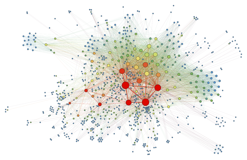
This article explains how to adapt Graph Neural Networks (GNNs) for image classification. It covers the process from converting images into graphs to updating the model’s parameters. I explore how message passing and global pooling can enhance spatial understanding and improve classification performance. I will begin by explaining the intuition behind GNNs and then examine how the model learns by breaking down the training loop.

---

1. Introduction

Convolutional Neural Networks (CNNs) are neural networks specialized in processing grid-structured data, such as images. As discussed in my previous article, they perform very well for image classification but do not fully account for complex relationships between distant pixels. This is where Graph Neural Networks (GNNs) come into play, allowing nearby pixels to exchange information, thereby improving the overall understanding of the image. In this article, I will begin by explaining the intuition behind GNNs and then examine how the model learns by breaking down the training loop.

The workflow looks like this:

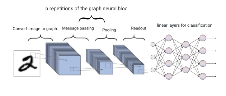
We start with an image that we convert to a graph. Then, we have multiple repetitions of the neural graph block (depending on the architecture for the specific application). Next, we have the readout, which transforms the graph-represented data into data the linear classifier can process. Finally, we get a prediction, which we will backpropagate on.

1. Graph Structure

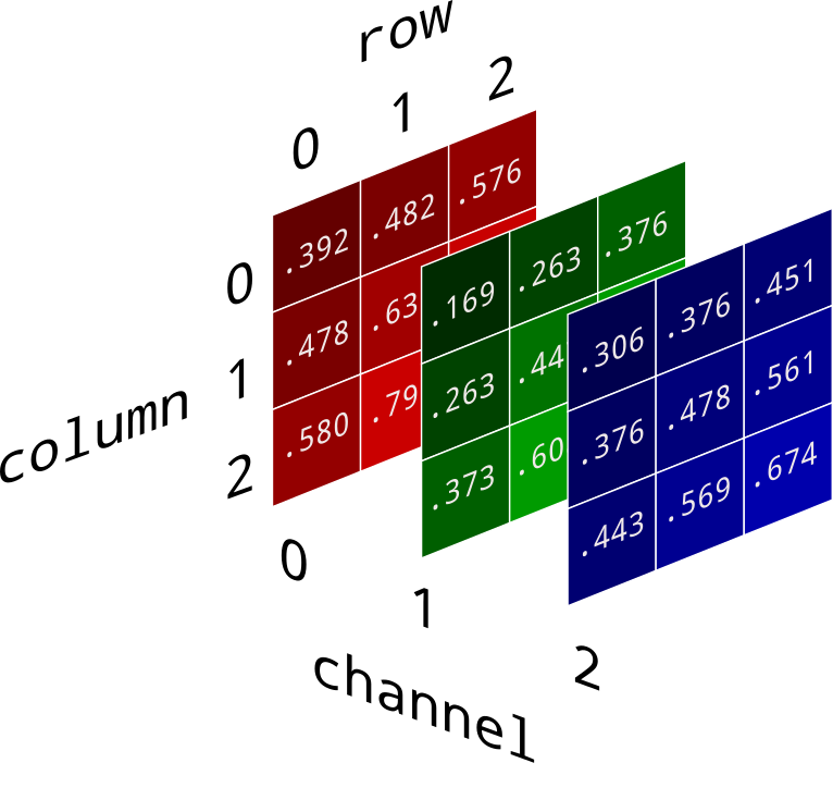
To start, the images need to be converted into graphs. RGB images are represented by three matrices, each corresponding to the intensity of a specific color as shown here:

A graph is a data structure made up of nodes connected by edges.

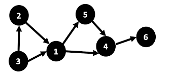
Our image, represented by the three matrices, is converted into a graph by creating one node for each pixel, with the three color values at that position and linking it to nearby pixels (creating the edges). This process can become very heavy because even small images have a lot of nodes (width x length). To solve this, we can use Super pixels to group local information from multiple pixels into one node, reducing the number of nodes. Another way to represent the image with a graph is to link the most similar super pixels using KNN clustering.

After this, we have a matrix with the values and an adjacency matrix representing the edges. (We are working with an undirected graph)

---

2. Message Passing

Once the image is turned into a graph, the nodes need to share information with their neighboring nodes. This process is called message passing. Message passing means that connected nodes exchange information. The new enriched node (repeated for every node) is obtained with the following expression:

The features of neighboring nodes are aggregated by calculating the average of the neighboring node features (which is the normalized):

This aggregation is weighted by the weight matrix W^(k), determining the relative importance of each feature. Then, the initial node features are added, weighted by a bias B^(k). Finally, the result is passed through a non-linear function f^(k), allowing the model to handle non-linear problems.

The Graph Neural block can be visualized like this:

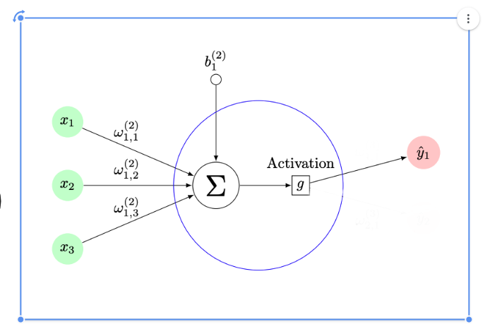
Here the green circles represent neighboring nodes aggregated with weight matrix W^(k) (represented by w1, w2,w3) and the bias ( B^(k)} (represented by b1 in the diagram), then passed through the activation function f^(k) (represented by g ).

---

3. Training Loop

3.1 Graph Neural Block

After converting the initial image into a graph, training begins with a sequence of Graph Neural blocks. These blocks consist of message-passing layers, as defined above, combined with Pooling layers. Pooling layers identify the most important nodes for understanding the graph by assigning each a score using an MLP (as detailed below). We then select the top ( K ) nodes (discarding the others) to eliminate noise and reduce computational load.

$$\text{score}(v_i) = W_2 \cdot \sigma(W_1 \cdot h_i + b_1) + b_2$$

Where:

• W1: Weight matrix for the first hidden layer

• b1: Bias vector for the first hidden layer

• sigma: Activation function (e.g., ReLU)

• W2: Weight matrix for the output layer

• b2: Bias vector for the output layer

---

3.2 Readout

After several iterations of Graph Neural blocks, the graph’s nodes are synthesized into a vector via global pooling, also known as Readout. This is done by taking the average, maximum, or sum of each node's features (a hybrid method or attention mechanism is also possible) to obtain a vector. This step is shown in the blue rectangle in the workflow. From here, the vector is passed through linear classification layers (as in a traditional CNN) to obtain a final probability for each class (illustrated by the nodes to the right of the Readout in the workflow).

---

3.3 Loss

Once predictions are made, we assess their quality with a loss function, representing the distance between the predictions and reality via a value. For binary classification tasks, Binary Cross Entropy Loss (BCE) is effective.

$$\text{BCE} = -\frac{1}{N} \sum_{i=0}^{N} \left( y_i \cdot \log(\hat{y}_i) + (1 - y_i) \cdot \log(1 - \hat{y}_i) \right)$$

Where:

• N: Total number of samples

• yi: True class label (0 or 1) for sample ( i )

• yˇi: Predicted probability that sample ( i ) belongs to class 1

---

• When yi = 1: BCE heavily penalizes if yˇi is close to 0 (wrong prediction), as (log(yˇi)) tends toward -infinity when yˇi approaches 0.

• When yi = 0: BCE heavily penalizes if yˇi is close to 1, as log(1 - yˇi) tends toward -infinity when yˇi approaches 1.

---

4. Backpropagation

Gradient Calculation

Gradients of the loss are calculated with respect to each parameter using the chain rule, which allows decomposing the gradient of a composite function into a product of simpler gradients. This enables determining each weight's influence on the loss.

For a weight ( w ), the gradient of the loss with respect to this weight is denoted

$$\frac{\partial L}{\partial w}$$

This gradient indicates the direction and magnitude of the necessary change to reduce the loss.

The chain rule is mathematically expressed as follows:

$$\frac{\partial L}{\partial w} = \frac{\partial L}{\partial y} \cdot \frac{\partial y}{\partial w}$$

where ( y ) is an intermediate variable dependent on weight ( w ).

---

Parameter Update

Once the gradients are computed, the model’s parameters are updated to minimize the loss. This is typically done using the gradient descent algorithm:

$$a_{n+1} = a_n - \lambda \nabla P$$

Where:

• an: Current model parameters at iteration n

• lambda: Learning rate, a hyperparameter controlling the update step size

• nabla P: Gradient of the loss with respect to the parameters

Each weight ( w ) is updated as follows:

$$w_{n+1} = w_n - \lambda \frac{\partial L}{\partial w}$$

By repeating this process over many iterations, the weights are adjusted to minimize the loss, thereby training the model.

---

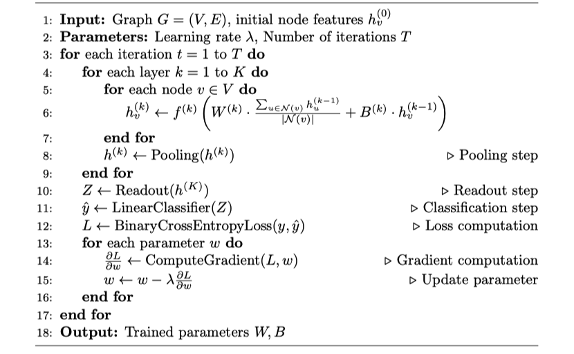
Now that we’ve looked into the steps of the workflow, here is the pseudo-code of the process

5. Algorithm Pseudo-code

Algorithm 1: Training Graph Neural Networks

---

In conclusion, we have seen how GNNs can be used for image classification. By converting images into graphs, using message passing, and applying global pooling techniques, GNNs can capture both local and long-range spatial dependencies. This enhances the model’s ability to recognize patterns and features that CNNs might miss.

The training process, from Graph Neural blocks to pooling and readout layers, ensures that the model systematically extracts important information, leading to more accurate predictions. As backpropagation and parameter updates refine the model, GNNs become increasingly skilled at classifying images with greater precision.

You can find an implementation on my github here.

If something wasn’t clear, if you want to expand on a topic, or if you just want to chat, feel free to reach out in the comments or here. Thanks for reading!