Introduction to Classification Models: Exploring Logistic Regression
 Omkar Kasture
Introduction
In this Article, we’ll be diving into three important classification models:
Logistic Regression
K-Nearest Neighbors (KNN)
Linear Discriminant Analysis (LDA)
As mentioned earlier, there are two types of prediction problems:
Regression Problems: Where the dependent variable (the one we want to predict) is continuous. An example would be predicting house prices, which we’ve explored before using linear regression.
Classification Problems: Here, the dependent variable is categorical, meaning we're predicting categories. For instance: Will a football player score a goal or not?, Does a patient have a heart issue or not?, Will it rain tomorrow or not?
For such classification problems, we use models like Logistic Regression, KNN, and LDA.
Used dataset
The dataset we’ll use is similar to our previous regression task (predicting house prices). However, this time, our goal is to predict the selling potential of a property. Based on past property transactions, we’ll predict whether a property will be sold within three months or not.
The dependent variable in our analysis is the sold variable, which contains values of either 0 or 1.
1means the property was sold within three months.0means it wasn’t.
The other variables in the dataset remain the same, except for the price variable, which is now an independent variable representing the asking price of the property.
Key Points to Remember:
The dataset is preprocessed, so you don’t need to worry about missing values, outliers, or other data cleaning steps.
The dataset is inspired by the Boston Housing dataset, commonly used for analysis, but it’s not real data, so don't take the results too seriously!
Click: GitHub repository for dataset and code
import pandas as pd
import numpy as np
import seaborn as sns

df = pd.read_csv('house_sold.csv', header=0)
df.head(5)
Logistic Regression
Why not linear regression for classification?
Let’s dive into our first classification technique: Logistic Regression.
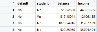
In above dataset, for example, we have three predictor variables: student, balance, and income, and the response variable, default (whether a person defaulted on their credit or not). The default variable is coded as 0 for no default and 1 for default.
If we were to run a simple linear regression using balance as the only predictor variable, we would obtain a straight line predicting the probability of default. We could set a boundary value, say 0.2, and classify anything above this threshold as 1 (default) and anything below as 0 (no default).
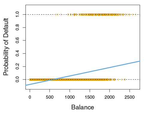
However, using linear regression for classification poses a significant problem: it can produce negative probabilities, which are not meaningful. Probabilities must lie between 0 and 1, and that's where logistic regression comes in.
Logistic regression solves this problem by using a logistic function, also known as the sigmoid function. This function maps any real-valued number into a range between 0 and 1, making it ideal for modeling probabilities. It transforms our linear equation into a curve that looks like an "S" shape, known as the logistic curve.
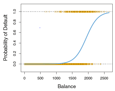
The logistic function can be expressed as

Estimating the Coefficients: Maximum Likelihood Estimation
Now, to build a logistic regression model, we need to estimate the values of β0 and β1. In linear regression, we use the Ordinary Least Squares (OLS) method, but in logistic regression, we use a technique called Maximum Likelihood Estimation (MLE).
The idea behind MLE is simple:
If a person defaults (i.e., the response variable is 1), we want the predicted probability P(X) to be as close to 1 as possible.
If a person does not default (i.e., the response variable is 0), we want P(X) to be as close to 0 as possible.
The MLE method maximizes the likelihood of these conditions, giving us the best estimates for our coefficients.
Training Simple Logistic Model

Let’s now train a simple logistic regression model using price as the predictor and Sold as the target variable.
First, import the necessary libraries and prepare your data:
# Importing necessary libraries
from sklearn.linear_model import LogisticRegression

# Define predictor and target variables
x = df[['price']]  # Predictor
y = df['Sold']     # Target variable
Next, instantiate and fit the logistic regression model:
# Initialize the Logistic Regression model
clf_lrs = LogisticRegression()

# Fit the model
clf_lrs.fit(x, y)
After fitting the model, you can extract the coefficients and intercept:
# Coefficient (B1)
clf_lrs.coef_

# Intercept (B0)
clf_lrs.intercept_
These values correspond to the β1 (coefficient) and β0 (intercept) in the logistic regression equation:

Now, you can use these β0 and β1 values in the logistic regression equation to predict the probability of Sold based on price.
y_pred = clf_lrs.predict(x)
y_pred
Output
We can do same using statsmodel.api
Logistic Regression with multiple predictors
The logistic regression equation for multiple predictors is:

Now lets train a logistic regression model using all available predictor variables to predict whether the property was sold within three months.
First, we prepare the data, selecting all columns except the target variable Sold as predictors:
# Define predictors and target variable
x = df.loc[:, df.columns != 'Sold']  # All columns except 'Sold'
y = df['Sold']  # Target variable
Next, instantiate and fit the logistic regression model:
# Initialize the Logistic Regression model
clf_lr = LogisticRegression()

# Fit the model
clf_lr.fit(x, y)
Once the model is trained, you can obtain the coefficients and intercept:
# Coefficients (B1, B2, ..., Bn)
clf_lr.coef_

# Intercept (B0)
clf_lr.intercept_
coefficients
intercept
These coefficients and intercept can be plugged into the logistic regression equation, where each predictor variable has its corresponding coefficient.
Finally, we predict the target variable (Sold) using the model:
# Predict the 'Sold' values
y_pred = clf_lr.predict(x)

# Display the predicted values
y_pred
y_pred
This will give you the predicted values for whether each property will be sold within three months based on all predictors.
Changing the Probability Threshold in Logistic Regression
In logistic regression, the default decision boundary or threshold for classification is 0.5, meaning if the predicted probability of being sold is 0.5 or greater, the prediction is 1 (sold), otherwise 0 (not sold).
However, you can adjust this threshold. For example, if you want to classify a property as "sold" if the probability is at least 0.3, here's how you can do that:
Step 1: Get Probabilities for Each Class
First, we can use clf_lr.predict_proba(x) to get the probabilities of each property being in either of the two classes (0: Not Sold, 1: Sold). The predict_proba() method returns a 2D array, where:
[:,0]contains the probabilities for class0(Not Sold),[:,1]contains the probabilities for class1(Sold).
# Get the probabilities for both 'Not Sold' (0) and 'Sold' (1)
proba = clf_lr.predict_proba(x)

# View the probabilities for class 'Sold' (1)
proba[:, 1]  # These are the probabilities of the property being sold
Step 2: Adjust the Threshold to 0.3
Next, you can classify properties as "sold" if the probability is greater than or equal to 0.3:
# Set a new threshold of 0.3 for being classified as 'Sold'
y_pred_03 = (proba[:, 1] >= 0.3)

# Print the new predictions
y_pred_03
y_pred_03
Confusion Matrix
The confusion matrix is a table used to evaluate the performance of a classification model. It compares the actual target values with the model’s predicted values and summarizes the results in four categories
| predicted negative | predicted positive | |
| actually negative | true negative (TN) | false positive (FP) |
| actually positive | false negative (FN) | true positive (TP) |
True Negative (TN) or Specificity:
The property was not sold, and the model correctly predicted that it wasn’t sold. This is the model's specificity.
False Positive (FP):
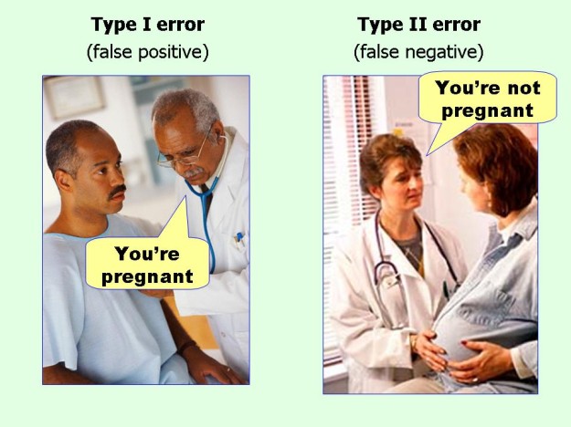
The property was not sold, but the model incorrectly predicted that it was sold. This is known as a Type I error or false alarm.
It reflects 1 - specificity (false positive rate).
False Negative (FN):
The property was sold, but the model predicted that it wasn’t sold. This is a Type II error or missed detection.
True Positive (TP):
The property was sold, and the model correctly predicted that it was sold. This indicates the model's sensitivity or power, which is the ability to correctly identify sold properties.
from sklearn.metrics import confusion_matrix

confusion_matrix(y, y_pred)
Output
Performance measure of classification model
| predicted negative | predicted positive | |
| actually negative | true negative (TN) | false positive (FP) |
| actually positive | false negative (FN) | true positive (TP) |
Accuracy: This represents the overall proportion of correct predictions.

Precision: Precision measures how many of the predicted positive classes (Sold) were actually correct. Maximizing precision means minimizing the loss.

Recall: Recall tells us how many actual positive classes (Sold) were correctly identified by the model. Maximizing precision means maximizing profit.

F1 Score (Harmonic Mean of Precision and Recall): F1 score gives a balanced measure of precision and recall.

from sklearn.metrics import precision_score, recall_score, accuracy_score

# Confusion matrix
cm = confusion_matrix(y, y_pred)
print(cm)

# Accuracy
accuracy = accuracy_score(y, y_pred)

# Precision
precision = precision_score(y, y_pred)

# Recall (Sensitivity)
recall = recall_score(y, y_pred)
This blog introduced classification models, focusing on logistic regression. In the next one, we’ll explore LDA, KNN, and logistic regression using the train_test_split method.
Keep Learning!
Subscribe to my newsletter
Read articles from Omkar Kasture directly inside your inbox. Subscribe to the newsletter, and don't miss out.
Written by

Omkar Kasture
Omkar Kasture
MERN Stack Developer, Machine learning & Deep Learning