Introduction

In the first part, we explored what a classification model is, using logistic regression as an example, along with the confusion matrix and different performance evaluation methods. In this article, we'll dive into two additional classification models: LDA and KNN algorithms.

First we will see implementation of classification models one by one.

Click: dataset and code for classification algorithms

Implementation of Logistic Regression:

Dataset: Import libraries and dataset

import pandas as pd
import numpy as np
import seaborn as sns

df = pd.read_csv('house_sold.csv', header=0)

Train Test Split

from sklearn.model_selection import train_test_split
X_train, X_test, Y_train, Y_test = train_test_split(x,y, test_size = 0.2, random_state=0)

print(X_train.shape, X_test.shape, Y_train.shape, Y_test.shape)

Model Building and Training

clf_LR = LogisticRegression()
clf_LR.fit(X_train, Y_train)

Assessing Model Performance

from sklearn.metrics import accuracy_score , confusion_matrix
y_test_pred = clf_LR.predict(X_test)
confusion_matrix(Y_test, y_test_pred)
accuracy_score(Y_test, y_test_pred)

As this is random dataset and not a real world data, the accuracy is low. But working with real world true dataset will give you proper accuracy.

Linear Discriminant Analysis (LDA)

In contrast to logistic regression, Linear Discriminant Analysis (LDA) is often the preferred technique when the response variable has more than two categories. LDA is based on Bayes' theorem and allows for easy interpretation of how different variables impact the output.

Conditional Probability and Bayes Theorem

Suppose we have a class of students, categorized by height (low, medium, and high) and fitness level (fit or not fit). Now, we aim to predict whether a student is fit given that their height is medium. This is conditional probability, as it is based on the precondition that the height is medium.

In above example, if there are 40 students of medium height, with 15 of them being fit, the probability of being fit given medium height is 15/40​.

Bayes' theorem helps calculate the probability of an event by considering prior knowledge of related events. If we want to find the probability that a student is both medium-heighted and fit, we can calculate it in two ways:

1. By first calculating the probability of being fit among medium-heighted students 15/40 and multiplying it by the probability of being medium-heighted overall 40/100. This gives 15/100​.

2. Alternatively, we can calculate the probability of having medium height among fit students 15/48 and multiply it by the probability of being fit overall 48/100. This also results in 15/100​.

Thus, Bayes' theorem allows us to calculate the same conditional probability using different perspectives.

What is LDA?

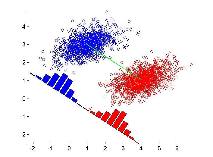
Linear Discriminant Analysis (LDA) is a classification technique used to find a linear combination of features that best separates different classes.

In LDA, continuous predictor variables are assumed to be normally distributed. For example, if we consider heights of students, they should follow a normal distribution. If this assumption holds true, LDA performs very well. However, if the assumption doesn't match reality, the accuracy may decrease. Nevertheless, in many real-world cases, this assumption holds, making LDA a reliable and powerful model.

To summarize, LDA calculates the probability of each observation belonging to a group and assigns the observation to the group with the highest probability.

Implementation of LDA

#import
from sklearn.discriminant_analysis import LinearDiscriminantAnalysis
# create object and train model
clf_LDA = LinearDiscriminantAnalysis()
clf_LDA.fit(X_train, Y_train)

#prediction
y_test_pred_LDA = clf_LDA.predict(X_test)

#performance assessment
confusion_matrix(Y_test, y_test_pred_LDA)
accuracy_score(Y_test, y_test_pred_LDA)

….Check for precision, recall, f1-score

K Nearest Neighbors ( KNN )

What is KNN?

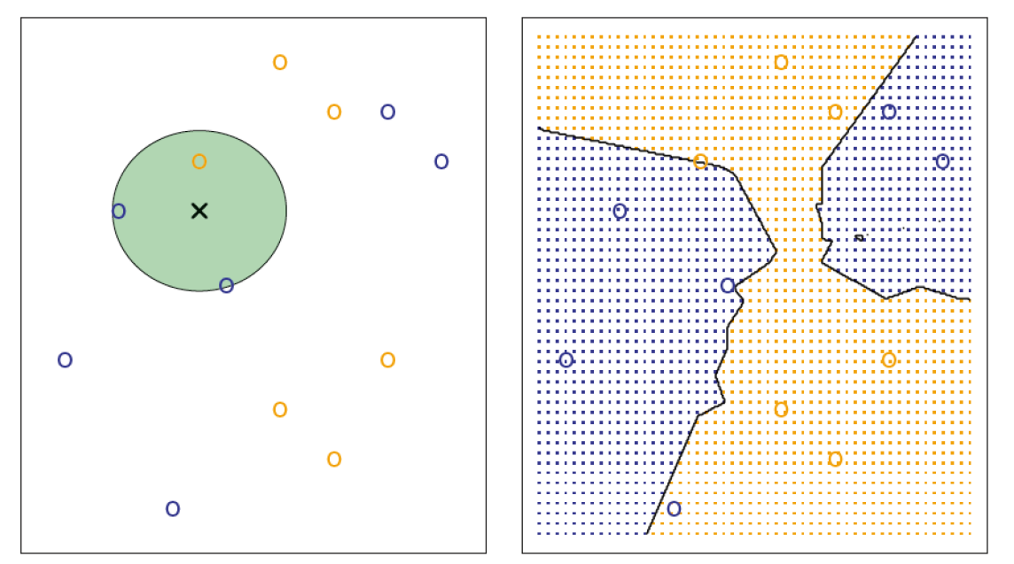
KNN is non-parametric supervised learning classification algorithm that assigns a class to a given observation based on the classes of its nearest neighbors, relying on conditional probabilities for classification.

• KNN is an instance-based learning algorithm, meaning it doesn't learn a fixed model from the training data. Instead, it stores the entire training dataset and makes decisions based on the local neighborhood of a point (nearest k neighbors).

• Being non-parametric means that KNN does not make any assumptions about the underlying distribution of data. This allows it to adapt to complex patterns in data, unlike parametric methods that assume a specific functional form (e.g., linear regression).

• In Simple words, It plot the data and for a observation it assigns the class same as the class of it’s neighbor observations.

How KNN Works?

Choosing the Number of Neighbors (k)

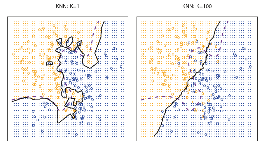
The choice of k is crucial.

• Low k (e.g. k=1): The model is highly sensitive to noise in the data, as it will classify a point based solely on the closest single neighbor. This can lead to overfitting.

• High k: A larger k smooths the decision boundary, making it less sensitive to noise, but it may also underfit the data if it's too large.

Voting Mechanism

KNN uses a voting mechanism to assign the class to a new observation:

• Majority Voting: Each neighbor votes for its class, and the class with the most votes is assigned to the observation.

• Weighted Voting: Neighbors closer to the observation have more influence than those further away, often done by weighting distances inversely

Why we need to standardize data?

• Feature Scaling: Since KNN relies on distance calculations, the scale of features significantly affects performance. For example, in a dataset with features like salary (in thousands) and age (in years), the salary will dominate the distance measure.

• Standardization: This is a common approach to scale features. It transforms each feature to have a mean of 0 and a standard deviation of 1.

  

  μ is the mean and σ is the standard deviation of the feature.

Choosing the Optimal k (Cross Validation)

The optimal k is typically determined through cross-validation:

• Cross-Validation: A technique where the dataset is split into training and validation sets multiple times to assess model performance. The k that yields the lowest validation error is often chosen.

• Error Analysis: Both training and test errors should be monitored. A small k may show low training error but high test error, indicating overfitting. Conversely, a large k might perform poorly on both, indicating underfitting.

Standardization of Features in Python

We Use the StandardScaler from the sklearn.preprocessing module in Python’s scikit-learn library to standardize the features of training and test datasets.

1. Importing the StandardScaler

    from sklearn import preprocessing
   

2. Creating a StandardScaler instance and fitting it to the training data

    scaler = preprocessing.StandardScaler().fit(X_train)
   

   • StandardScaler() initializes a new instance of the StandardScaler class.

   • The fit() method calculates the mean and standard deviation of the features in the training data (X_train). This is done to learn the parameters needed for scaling (i.e., the mean and standard deviation).

3. Transforming the training and testing data

    X_train_s = scaler.transform(X_train)
    X_test_s = scaler.transform(X_test)
   

   Each feature is standardized using the formula:

   

   where x is the original value, μ is the mean of the feature (calculated during fitting), and σ is the standard deviation of the feature (also calculated during fitting).

4. standardized data

    print(X_train_s)
    print(X_test_s)
   

   X_train_s

   (array([[ 0.44572353, -0.70492455, -0.42487874, ..., -0.48525664, -0.40529635, 1.3293319 ], [-0.09643431, -0.04487755, -1.24185891, ..., -0.48525664, 2.4673304 , -0.75225758], [ 0.478253 , -0.88675963, -1.11148974, ..., -0.48525664, -0.40529635, -0.75225758], ..., [-0.36751323, -0.15941933, -0.0772276 , ..., -0.48525664, 2.4673304 , -0.75225758], [-0.64943531, -0.60326872, -0.93766417, ..., -0.48525664, -0.40529635, 1.3293319 ], [ 0.05536988, -1.01275558, -0.3988049 , ..., -0.48525664, -0.40529635, 1.3293319 ]]),

each data is standardized such that mean of each column is 0 and standard deviation is 1.

means=np.mean(X_train_s, axis=0)
print(means)
std_dev = np.std(X_train_s, axis=0)
print(std_dev)

Building KNN model

from sklearn.neighbors import KNeighborsClassifier

clf_knn_1 = KNeighborsClassifier(n_neighbors=1) # k=1
clf_knn_1.fit(X_train_s, Y_train)

confusion_matrix(Y_test, clf_knn_1.predict(X_test_s))
accuracy_score(Y_test, clf_knn_1.predict(X_test_s))

Grid Search CV

You can build more KNN models for different model for different value of k, and then choose best model out of them. But instead, we can build all this models at once using grid search cv.

Import Required Libraries:

from sklearn.model_selection import GridSearchCV
from sklearn.neighbors import KNeighborsClassifier
from sklearn.metrics import confusion_matrix, accuracy_score

Set Up the Parameter Grid: We define the range of k values we want to test.

params = {'n_neighbors': [1, 2, 3, 4, 5, 6, 7, 8, 9, 10]}

Initialize GridSearchCV: We create an instance of GridSearchCV, passing in the KNN classifier and the parameter grid.

grid_search_cv = GridSearchCV(KNeighborsClassifier(), params)

• KNeighborsClassifier(): This initializes the KNN classifier.

• params: This dictionary specifies the values of k to test.

Fit the Model:

grid_search_cv.fit(X_train_s, Y_train)

During this process, GridSearchCV will evaluate each model using cross-validation to determine which k gives the best performance.

Parameters: After fitting, you can access the best value of k found during the search

best_k = grid_search_cv.best_params_

Optimized KNN Model: The best KNN model can be accessed using

optimized_KNN = grid_search_cv.best_estimator_

Make Predictions:

y_test_pred = optimized_KNN.predict(X_test_s)
confusion_matrix(Y_test, y_test_pred)
accuracy_score(Y_test, y_test_pred)

Conclusion

In conclusion, classification models like Logistic Regression, Linear Discriminant Analysis (LDA), and K-Nearest Neighbors (KNN) offer powerful tools for tackling various classification problems.

While logistic regression is effective for binary outcomes, LDA excels when dealing with multiple classes by leveraging Bayes' theorem for interpretation.

KNN provides a flexible, non-parametric approach that can adapt to complex data distributions, especially when properly standardized and optimized.

The upcoming blog will focus on decision trees. Until then, happy learning!