Introduction

We’ve already explored some basic machine learning models, and now, we’ll dive into Decision Trees, one of the most popular and powerful machine learning techniques.

Decision trees are not only easy to interpret but also highly effective at predicting complex patterns in data. Their combination of interpretability and accuracy makes them popular in both the business and data science communities.

What We'll Cover?

We will cover all concept of decision tree in three parts.

• Regression Trees: Focus on predicting continuous outcomes.

• Classification Trees: Handling categorical predictions.

• Tree Pruning: Controlling the complexity of the tree.

• Advanced Ensemble Techniques: Bagging, Random Forest, and Boosting methods for enhanced performance.

In this section, we will dive into Regression Tree and the logic behind decision trees.

What is a Decision Tree?

A decision tree is a popular decision support tool that uses a tree-like structure to model decisions and their possible consequences, including chance outcomes, costs, and utility.

It visually represents the decision-making process, where each node represents a decision or a test on an attribute, and each branch represents the outcome of that decision. The leaf nodes at the end of the tree show the final output or prediction.

In machine learning, a decision tree works as a flowchart-like model that uses a series of conditional control statements to split data into smaller and smaller subsets, ultimately helping in classification or regression tasks.

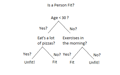
In a decision tree, the goal is to split the population into distinct regions or segments, where each region represents a group of observations with similar characteristics based on predictor variables. In this example, the tree ultimately divides the data into four regions, each of which classifies individuals as either "unfit" or "fit" based on their characteristics. Each split refines the classification by focusing on key predictors that help distinguish between these groups.

What is a Regression Tree?

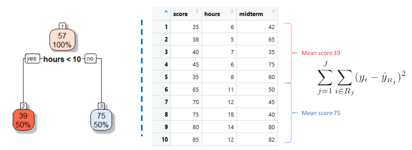
A Regression Tree works by splitting the predictor space into distinct regions and making predictions based on the average response in each region.

Steps in Building a Regression Tree:

1. Dividing the Predictor Space:

   We divide the predictor space (the set of possible values for X1,X2, . . …,Xp ) into J distinct and non-overlapping regions, R1,R2, . . . , RJ .

2. Prediction:

   For every observation that falls into a particular region Rj​, the prediction is the mean of the response values of all training observations in that region.

3. Goal:

   The aim is to minimize the Residual Sum of Squares (RSS), which is the total squared difference between actual and predicted values.

Process:

1. Consider All Predictors and Cut Points:

   The tree evaluates all predictor variables and all possible cut points to determine where to split the data.

2. Calculate RSS:

   For each split, the tree calculates the RSS to measure the error in predictions.

3. Select the Best Split:

   The split that gives the least RSS (minimizing error) is selected.

4. Continue Splitting:

   This process continues recursively until a stopping criterion (e.g., minimum node size or maximum depth) is met.

By iteratively splitting the predictor space and minimizing RSS, the tree creates a model that can predict continuous outcomes.

Why Controlling Tree Growth is Needed?

We need to control the growth of a decision tree to avoid overfitting. Overfitting happens when a model becomes too complex and starts to memorize the training data instead of learning general patterns. This makes the model perform very well on the training data but poorly on new, unseen data.

What is Overfitting (in simple words)?

Think of it like studying for an exam. If you only memorize specific questions and their answers, you'll do great if the same questions appear in the exam. But if the questions are different, you’ll struggle because you didn’t understand the concepts. Overfitting is like that—your decision tree learns the exact data you gave it but doesn’t do well with new data because it didn’t capture general trends.

Ways to Control Tree Growth

1. Minimum Number of Observations to Split a Node:

   • Set a limit for how many observations (data points) must be in a node before it's split. If there aren’t enough, the split won’t happen.

   • This avoids making splits on very small groups, which can lead to overly specific branches that don’t generalize well.

2. Minimum Number of Observations at a Leaf Node:

   • Ensure that after a split, each leaf (final node) has a minimum number of observations. If a split results in too few observations, the tree stops growing there.

   • It prevents the tree from creating too many tiny, specialized regions.

3. Maximum Depth of the Tree:

   • Limit how deep (complex) the tree can go. A shallow tree makes fewer splits, resulting in a simpler model.

   • This avoids making the tree too detailed, which could lead to memorizing the training data instead of learning useful patterns.

These methods help the decision tree focus on general patterns in the data instead of getting too detailed, making it better at handling new, unseen data.

Implementing Regression Tree

We’ll be using a movie dataset to build our regression tree model, where the goal is to predict the box office collection (revenue) for a movie before it’s released. The dataset includes 17 predictor variables.

Get Dataset and Code : GitHub Link

Step 1: Data Preprocessing

import numpy as np
import pandas as pd
import seaborn as sns
import matplotlib.pyplot as plt

df= pd.read_csv("Movie_regression.csv", header=0)
df.head()
df.info()

time_taken has some null values

# impute mean value of time_taken in all null
df['Time_taken'].fillna(value= df['Time_taken'].mean(), inplace = True)

Create dummy variables for categorical data, 3D_available and Genre

df = pd.get_dummies(df, columns =[ "3D_available","Genre"], drop_first=True)
df['3D_available_YES'] = df['3D_available_YES'].astype(int)
df['Genre_Comedy'] = df['Genre_Comedy'].astype(int)
df['Genre_Drama'] = df['Genre_Drama'].astype(int)
df['Genre_Thriller'] = df['Genre_Thriller'].astype(int)

Step 2: Test Train Split

X = df.loc[: , df.columns != "Collection"]
Y = df['Collection']

from sklearn.model_selection import train_test_split
X_train, X_test, Y_train, Y_test = train_test_split(X,Y, test_size=0.2, random_state=0)

Step 3: Model Building

from sklearn import tree
regtree = tree.DecisionTreeRegressor(max_depth=3)
regtree.fit(X_train, Y_train)

y_train_pred = regtree.predict(X_train)
y_test_pred = regtree.predict(X_test)

Step 4: Model Performance

We’ve built our tree regressor model and predicted values for both the training and test datasets. Now, it’s time to evaluate performance using two key metrics: Mean Squared Error (MSE) and R-squared (R²).

MSE measures the average squared deviations of predicted values from actual values, while R² indicates the model's goodness of fit, ranging from 0 (no fit) to 1 (perfect fit).

Good models typically have R² values between 0.42 and 0.80, with values above 0.80 indicating excellent performance.

from sklearn.metrics import mean_squared_error, r2_score
mean_squared_error(Y_test, y_test_pred)
r2_score(Y_train, y_train_pred)
r2_score(Y_test, y_test_pred)

mean_squared_error

94270653.74813624

r2_score for training data

0.8364651040556869

r2_score for testing data

0.707165453856755

Our training dataset has an R² value of 0.83, indicating strong performance. However, the test dataset's R² is 0.70. This drop is expected, as models generally perform better on training data, reinforcing the importance of evaluating test R² values for a reliable assessment of model performance.

Step 5: Plotting Regression Tree

dot_data = tree.export_graphviz(regtree, out_file=None, 
                           filled=True, rounded=True, 
                           special_characters=True)

from IPython.display import Image
import pydotplus
graph = pydotplus.graph_from_dot_data(dot_data)
Image(graph.create_png())

Controlling Tree Growth

You can control tree growth using various attributes in DecisionTreeRegressor function and check for more accuracy.

regtree1 = tree.DecisionTreeRegressor( max_depth = 3)

regtree2 = tree.DecisionTreeRegressor(min_samples_split = 40) 
# for further split min sample size should be 40

regtree3 = tree.DecisionTreeRegressor(min_samples_leaf = 25)  
# for further split min sample size of leaf should be 25

regtree4 = tree.DecisionTreeRegressor(min_samples_leaf = 25, max_depth=4)
#multiple conditions can be applied

In next blogs, We will see how to automate this process, how to pass multiple values of this hyper parameters and how to select the best model out of all these kinds of models that we are going to create. We will do that after our classification tree.

In this blog, we learned about decision trees, regression trees, and the importance of controlling their growth to prevent overfitting. We also explored various methods for managing tree complexity, including pruning techniques.

In the next part, we will delve into classification trees and ensemble techniques to enhance model performance.

Happy Learning!