In the previous part of this series, we explored and implemented regression trees while covering the concept of decision trees. If you directly reached to this blog, I recommend you to first read part-1 of decision tree, as all basics are covered in first part, and without basics this part will be a little confusing for beginners.

In this article, we’ll dive into using decision trees for categorical predictions, focusing on the decision tree classifier. Let's get started!

Decision Tree For Classification

Decision trees can be applied in two ways:

1. Regression Tree

   • Used for continuous, quantitative target variables.

   • Examples: predicting rainfall, revenue, or exam scores.

2. Classification Tree

   • Used for discrete, categorical target variables.

   • Examples: predicting categories like High vs. Low, Win vs. Loss, or Healthy vs. Unhealthy.

Prediction Methods:

• Regression:
  As discussed in part-1, The mean of the response variable is used as the prediction for each region.

• Classification:
  For Classification, The prediction is based on the mode (the most frequent category) within each region.

Splitting Methods:

Both regression and classification trees use recursive binary splitting to decide splits:

• Regression Trees use Residual Sum of Squares (RSS).

• Classification Trees use:

  1. Classification Error Rate

  2. Gini Index

  3. Cross Entropy (or Log Loss)

Splitting Methods for Classification Tree

Classification Error Rate

Classification error rate is the simplest metric for evaluating a classification decision. It measures the proportion of incorrect predictions made by the model in a given region.

where pk is the proportion of data points in the region that belong to class k.

It calculates the percentage of misclassified instances. However, it’s not as sensitive to the purity of the split compared to other metrics, making it less commonly used in practice.

Gini Index

The Gini Index (or Gini Impurity) measures the degree of impurity or disorder in a region. A low Gini Index indicates a region where most observations belong to a single class (i.e., it's more "pure").

where pk​ is the proportion of data points in class k in the region, and K is the total number of classes.

Example, If a node contains 80% instances of Class A and 20% of Class B, the Gini Index would be: Gini=1−(0.8×0.8+0.2×0.2)=0.32

• The Gini Index ranges from 0 (perfectly pure, all observations in a region belong to one class) to 0.5 (maximally impure, an even split between two classes).

• It encourages splits that create regions where one class dominates, which improves classification performance.

Cross Entropy (or Log Loss)

Cross Entropy (also known as Log Loss) is a measure of the uncertainty in predictions. It penalizes confident but incorrect predictions more than the Gini Index, making it a more sensitive measure of the purity of a split.

For example, If a node has 90% of Class A and 10% of Class B, the Cross Entropy would be: Cross Entropy=−(0.9*log⁡(0.9)+0.1*log⁡(0.1))=0.325

• Cross Entropy measures the amount of “information” needed to describe the uncertainty in the prediction.

• A lower Cross Entropy indicates higher purity of the split, where one class dominates.

• It is more sensitive to misclassifications than the Gini Index because it increases sharply for wrong predictions made with high confidence.

Advantages and Disadvantages of using Decision Tree for Classification

Advantages:

1. Easy to Explain: Decision trees are simple and intuitive, making them easy to understand for non-technical stakeholders.

2. Mimic Human Decision-Making: The tree structure mirrors human decision-making, making it easier to relate to compared to more complex models.

3. Visual Representation: Decision trees can be displayed graphically, allowing for easy interpretation, even by non-experts.

4. Handles Qualitative Predictors: Decision trees can work directly with categorical variables without needing to create dummy variables, simplifying the process.

Disadvantages:

1. Lower Predictive Accuracy: Decision trees often do not perform as well in terms of predictive accuracy compared to more sophisticated models.

Implementation of Decision Tree Classifier

Get Dataset and Code Here : github/decision_trees

Step 1: Data Preprocessing

import numpy as np
import pandas as pd
import seaborn as sns
import matplotlib.pyplot as plt

df= pd.read_csv("Movie_classification.csv", header=0)
df.head() # observe data 
df.info() #analyse data

# impute mean value of time_taken in all null
df['Time_taken'].fillna(value= df['Time_taken'].mean(), inplace = True)

#dummy variables creation
df = pd.get_dummies(df, columns =[ "3D_available","Genre"], drop_first=True)
df['3D_available_YES'] = df['3D_available_YES'].astype(int)
df['Genre_Comedy'] = df['Genre_Comedy'].astype(int)
df['Genre_Drama'] = df['Genre_Drama'].astype(int)
df['Genre_Thriller'] = df['Genre_Thriller'].astype(int)

#train test split
X = df.loc[: , df.columns != "Start_Tech_Oscar"]  
#iloc takes two parameters rows and columns ":" for all rows

Y = df['Start_Tech_Oscar']
from sklearn.model_selection import train_test_split
X_train, X_test, Y_train, Y_test = train_test_split(X,Y, test_size=0.2, random_state=0)

X_train.shape, X_test.shape, Y_train.shape, Y_test.shape

Step 2: Model Building

from sklearn import tree
clftree = tree.DecisionTreeClassifier(max_depth=3) 
clftree.fit(X_train, Y_train)

Step 3: Predictions and Performance Assessment

y_train_pred = clftree.predict(X_train)
y_test_pred = clftree.predict(X_test)

from sklearn.metrics import accuracy_score , confusion_matrix
confusion_matrix(Y_train, y_train_pred)
confusion_matrix(Y_test, y_test_pred)
accuracy_score(Y_test, y_test_pred)

accuracy_score

0.5490196078431373

Step 4: Plotting Tree

dot_data = tree.export_graphviz(clftree, out_file=None, 
                           filled=True,feature_names=X_train.columns)
from IPython.display import Image
import pydotplus
graph = pydotplus.graph_from_dot_data(dot_data)
Image(graph.create_png())

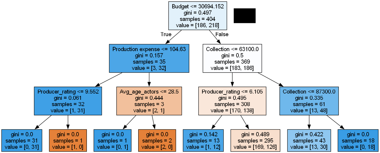
We can see, The gini Index is used as splitting method by default.

The accuracy achieved is 0.549, which is comparatively too less. There are two reasons behind the less accuracy. first the data we used is not real data, is is randomly generated.

But the second reason is more important, as we can see in tree most of regions have 0 entropy and samples=1 i.e. we created region for one data point. and that’s why the region is pure. But it may lead to incorrect prediction, because the tree is now overfitted.

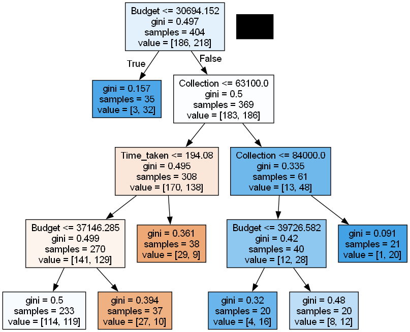
To avoid overfitting, we need to control growth of tree using various measures.

Controlling Tree Growth

clftree2 = tree.DecisionTreeClassifier(min_samples_leaf = 20, max_depth=4)
clftree2.fit(X_train, Y_train)
dot_data = tree.export_graphviz(clftree2, out_file = None, feature_names=X_train.columns, filled=True)
graph2=pydotplus.graph_from_dot_data(dot_data)
Image(graph2.create_png())

Conclusion

In this article, we explored how decision trees can be used for classification problems. However, a single decision tree may not always provide the best predictive accuracy due to its tendency to overfit the data. This is where Ensemble Methods comes in.

Why We Need Ensemble Methods?

• Improves Accuracy: By combining the predictions of multiple models, ensembling reduces the risk of overfitting and enhances overall performance.

• Reduces Variance: Decision trees are sensitive to small changes in the data, which can lead to high variance. Ensembling methods, like Bagging and Random Forest, help stabilize predictions.

• Balances Bias and Variance: Ensembling can balance out the high variance of decision trees and create more robust models.

In the next part, we will explore various ensembling techniques.

Happy Learning!