In previous parts of decision trees, we explored what are decision trees and how they can be used for regression as well as classification. In this blog we will see the problem with normal classification tree, and how to overcome it using various ensemble techniques.

Problem with normal decision tree?

In Decision Trees, one major issue is high variance. This means small changes in the training data can lead to very different tree structures. For instance, if you split your data into two halves and train two separate decision trees, the trees may look completely different.

Using a movie dataset, when I created two halves of the training data and trained regression trees on each, I saw two different trees. One tree split on the budget variable, while the other split on trailer views. The structures were different throughout.

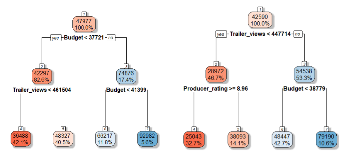
This high variance leads to unstable predictions based on the specific training data used. To reduce this variance and improve accuracy, a natural approach is to train multiple models on different subsets of the data. Then, by averaging their predictions, we can achieve a more stable and accurate result.

We'll discuss three popular ensemble techniques:

1. Bagging: This method trains multiple decision trees on all features of the dataset, but taking subset of data and combines their predictions for a more stable result.

2. Random Forest: A specific type of bagging, Random Forest adds randomness by selecting a subset of features for each tree, making it more robust.

3. Boosting: Unlike bagging, boosting trains trees sequentially. Each tree tries to correct the mistakes of the previous one, resulting in an improved model.

Ensemble Method-1: Bagging

Bagging is an ensemble method where we use all variables but create multiple training sets from a single dataset. and take average of all predictions.

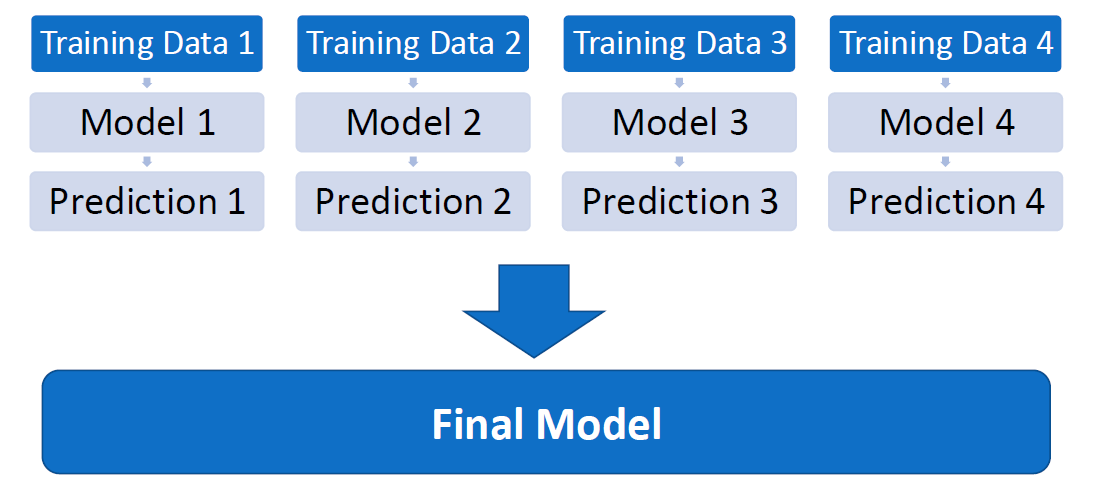
Principle of bagging:

The key idea is that if we divide total population into k samples (subsets of population), and each sample has variance σ², then the variance of the mean of each sample is σ²/n

So by averaging predictions, we reduce the overall variance. But since we don't have access to multiple training sets, we use bootstrapping.

Bootstrapping:

Bootstrapping involves creating multiple samples by randomly selecting data points with replacement from the original dataset.

Ex. 7 9 5 4 3 ==> Sample1 - 9 5 4 3 4, Sample2 - 7 9 5 4 7, Sample3 - 7 9 9 4 3

Through bootstrapping, we can create multiple training sets, each slightly different from the original one, which helps build diverse models.

Tree Growth:

When growing trees in bagging, we allow them to grow fully without pruning because pruning reduces variance by simplifying the tree.

Fully grown trees have low bias but high variance, meaning they can capture intricate patterns in the data without being overly simplified.

Since the main goal of bagging is to reduce variance, we don't prune the trees, even though each individual tree might overfit.

The averaging process across multiple high-variance trees smooths out the overfitting, reducing overall variance and improving prediction accuracy.

Final Prediction:

• For regression, where we're predicting continuous values, we take the average of the predicted values from all the individual trees. This averaging reduces the variance and gives a more stable prediction.

• For classification, where we're predicting categories or classes, we use a majority vote. Each tree predicts a class, and the class that appears most frequently across all trees is chosen as the final prediction.

Implementation of Bagging in Python

Guide : https://scikit-learn.org/sklearn.ensemble.BaggingClassifier.html

Dataset and code: https://github.com/omkar-2483/decision_trees

step-1: Create Decision Tree Classifier

from sklearn import tree
clftree = tree.DecisionTreeClassifier()

This imports the DecisionTreeClassifier from sklearn. We are creating a base classifier (clftree) which is a simple decision tree. This will serve as the model for each tree in the bagging ensemble.

Step-2: Setting up the Bagging Classifier

from sklearn.ensemble import BaggingClassifier
bag_clf = BaggingClassifier(estimator=clftree, n_estimators=1000, bootstrap=True, n_jobs=-1, random_state=42)

• estimator=clftree: Specifies that the base estimator (or model) used for bagging is the decision tree classifier we defined earlier.

• n_estimators=1000: This means we want to create an ensemble of 1000 decision trees. The predictions of these 1000 trees will be aggregated (using majority vote for classification).

• bootstrap=True: Enables bootstrapping, meaning that each of the 1000 decision trees will be trained on a random subset of the training data with replacement.

• n_jobs=-1: This allows the model to use all available CPU cores for parallel processing, speeding up the training process.

• random_state=42: Ensures reproducibility by setting the random number generator to a fixed seed.

Step-3: Training the Model

bag_clf.fit(X_train, Y_train)

It builds 1000 decision trees using bootstrapped samples of the training data.

Step-4: Evaluating the Model:

confusion_matrix(Y_test, bag_clf.predict(X_test))
accuracy_score(Y_test, bag_clf.predict(X_test))

accuracy-score

0.6176470588235294

We can see the accuracy in now increased from 54.90 % to 61.76 %.

Ensemble Method-2: Random Forest

Problem with Bagging: Correlated Trees

In bagging, all trees are built using all available predictor variables. This can lead to a problem:

• If there is a strong predictor in the dataset, most of the trees will use this predictor for the first split. As a result, many trees will look similar, producing correlated outcomes.

• When predictions from these highly correlated trees are averaged, it doesn’t reduce variance significantly.

Solution: Random Forest

Random Forest improves over bagging by reducing correlation between trees.

Instead of using all predictors for every tree, Random Forest selects a random subset of predictors for each tree.

This prevents every tree from relying on the same strong predictors, leading to more diverse and less correlated trees.

Process of Random Forest

The process is similar to bagging, but with one additional step:

• Randomly select m predictors from the total p predictors for each tree.

• Each tree uses different set of m predictors for making splits, resulting in a more diverse set of trees.

• If m==p (i.e., we use all predictors), Random Forest becomes equivalent to bagging.

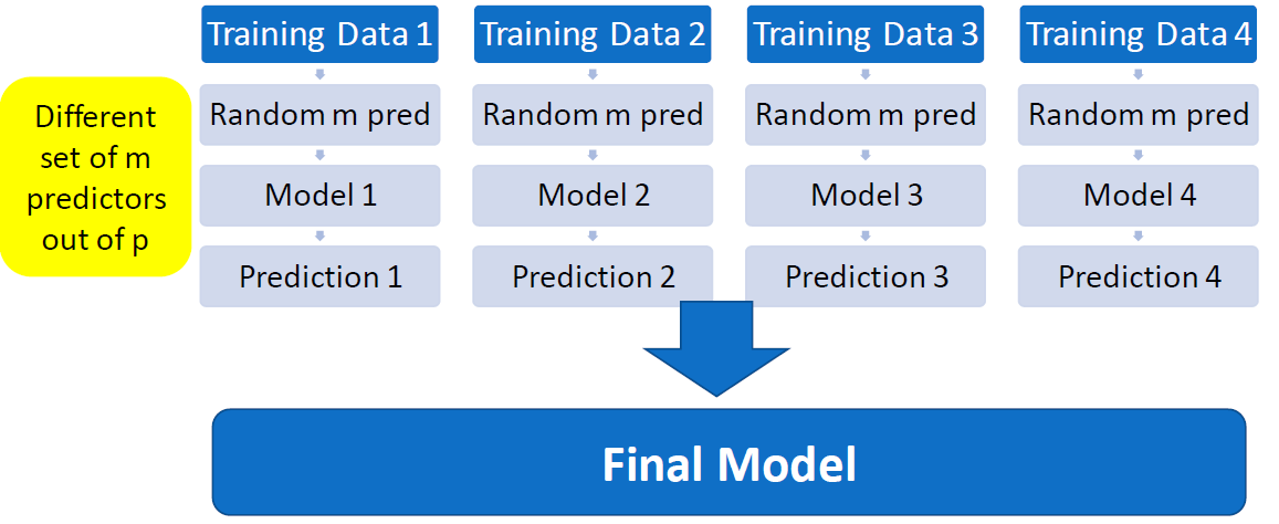
Choosing value of m: The number of predictors to use for each tree is an important decision.

• For regression: A common rule of thumb is to set m=p/3.

• For classification: Set m= sqrt(p).

Implementation of Random Forest in Python

Guide: https://scikit-learn.org/sklearn.ensemble.RandomForestRegressor.html

Dataset and code: https://github.com/omkar-2483/decision_trees

from sklearn.ensemble import RandomForestClassifier

rf_clf = RandomForestClassifier(n_estimators=1000, n_jobs=-1, random_state=42)
rf_clf.fit(X_train, Y_train)

confusion_matrix(Y_test, rf_clf.predict(X_test))
accuracy_score(Y_test, rf_clf.predict(X_test))

accuracy_score

0.6372549019607843

with random forest classifier we achieved accuracy of 63.72 %.

Note : In the RandomForestClassifier, you don't explicitly pass an estimator (like you do in Bagging Classifier) because RandomForestClassifier automatically uses decision trees as its base estimators.

In contrast, BaggingClassifier is a more generic method where you can specify any kind of estimator, such as decision trees, logistic regression, or SVM, by passing it to the estimator argument. But RandomForestClassifier is specifically designed to use decision trees internally, so you don't need to specify the estimator.

Parameters:

You can pass various parameters in RandomForestClassifier to optimize the performance further.

max_depth: Default: None

Maximum depth of the trees. If not set, trees will grow until all leaves are pure or until they cannot be split further.

min_samples_split: Default: 2

Minimum number of samples required to split an internal node. Can be an integer or a fraction of the total samples.

min_samples_leaf: Default: 1

Minimum number of samples required at a leaf node. Can smooth the model, especially in regression tasks.

max_features (m): Default: 1.0

Number of features to consider when looking for the best split:

• "sqrt": Square root of total features.

  "log2": Log base 2 of total features.

  float: A fraction of the total features.

  int: Fixed number of features.

• Smaller values add more randomness and help reduce correlation between trees.

bootstrap: Default: True

Whether to use bootstrap samples (sampling with replacement) to train each tree. If False, the whole dataset is used for every tree.

n_jobs: Default: None

Number of jobs to run in parallel. Set to -1 to use all available cores for faster computation.

random_state:

Controls randomness in bootstrapping and feature selection, ensuring reproducibility.

max_samples: Default: None

Number (or fraction) of samples to draw for each tree when bootstrap=True.

Grid Search to find best parameter values:

from sklearn.model_selection import GridSearchCV
# Features which are same for all trees are passed directly
rf_clf= RandomForestClassifier(n_estimators=250 , random_state=42)

params_grid = {"max_features": [4,5,6,7,8,9,10], 
               "min_samples_split": [2,3,10]}
grid_search = GridSearchCV(rf_clf, params_grid, n_jobs=-1, cv=5, scoring="accuracy")

grid_search.fit(X_train, Y_train)

Find best parameters and best estimator

grid_search.best_params_
cvrf_clf = grid_search.best_estimator_

confusion_matrix(Y_test, cvrf_clf.predict(X_test))
accuracy_score(Y_test, cvrf_clf.predict(X_test))

bestparams

{'max_features': 6, 'min_samples_split': 3}

Ensemble Method-3: Boosting

In boosting, we create multiple trees sequentially, with each tree learning from the mistakes of the previous one. Three key boosting techniques are Gradient Boosting, AdaBoost, and XGBoost.

Gradient Boosting

Gradient Boosting is an ensemble learning technique that builds models sequentially. Instead of training multiple independent models like in bagging (e.g., Random Forests), gradient boosting trains models that learn from the mistakes of previous models. It is primarily used for regression and classification tasks.

The idea behind Gradient Boosting is to improve a model by combining weak learners (typically shallow decision trees) sequentially, where each new learner focuses on the errors (residuals) made by the previous one.

How Gradient Boosting Works?

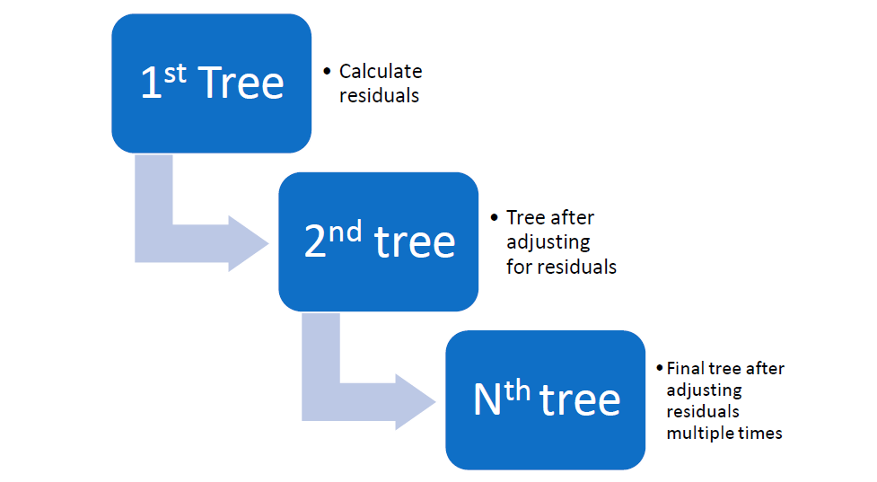
1. Initialize the Model: The algorithm starts by making an initial prediction, typically the mean (for regression) or the most frequent class (for classification). This becomes the baseline model.

2. Compute Residuals (Errors) : For each subsequent model, instead of predicting the actual target, the algorithm tries to predict the residuals (errors) from the previous model.

Residual = Actual value - Predicted value

3. Fit a Weak Learner: A new decision tree (or weak learner) is then trained on these residuals to predict the parts the previous model didn’t get right.

This tree is kept small and shallow, usually with a predefined maximum depth. The small size of the trees helps prevent overfitting.

4. Update the Model: The predictions of the new tree are scaled by a factor called the learning rate (shrinkage parameter) and added to the predictions of the previous trees. The learning rate controls how much influence each new tree has on the final model.

New Prediction = Old Prediction + (Learning Rate) * (New Tree’s Prediction)

5. Repeat: This process of computing residuals, fitting a new tree, and updating predictions is repeated multiple times for a predefined number of iterations (trees). With each iteration, the model focuses more on the areas where the previous models made mistakes.

Key Tuning Parameters in Gradient Boosting

1. Number of Trees (n_estimators): This is the total number of trees (iterations) used in the ensemble. A higher number of trees usually leads to better performance, but too many trees can lead to overfitting. The optimal number of trees is often found through cross-validation.

2. Learning Rate (Shrinkage Parameter Lambda): Controls how much each tree contributes to the overall model. A small learning rate makes the model learn slower but more cautiously, while a larger learning rate speeds up learning but can lead to overfitting. A typical range is between 0.01 and 0.1.

3. Tree Depth (max_depth): Smaller trees (low depth) reduce the risk of overfitting and force the model to learn simple patterns, while deeper trees can capture more complex patterns but risk overfitting. Even stumps (depth=1) can sometimes work well.

Limitations

1. Prone to Overfitting: If not properly tuned, the model can overfit, especially with too many trees or large tree depth.

2. Slow Training: Gradient boosting builds trees sequentially, so training can be slow compared to parallel methods like Random Forests.

3. Sensitive to outliers: Outliers can significantly affect the performance of gradient boosting, as it tries to minimize the residuals for all points.

Implementation in Python

Dataset and code: https://github.com/omkar-2483/decision_trees

rom sklearn.ensemble import GradientBoostingClassifier

gbc_clf2 = GradientBoostingClassifier(learning_rate=0.02, n_estimators=1000, max_depth=1)
gbc_clf2.fit(X_train, Y_train)

accuracy_score(Y_test, gbc_clf2.predict(X_test))

accuracy_score

0.6176470588235294

You can apply grid search to find best parameters for better accuracy.

AdaBoost (Adaptive Boosting)

AdaBoost (Adaptive Boosting) is an ensemble technique that builds multiple weak learners (typically decision trees) sequentially.

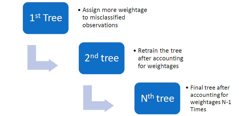
In each iteration, it focuses on the misclassified instances by increasing their weights, making the next tree pay more attention to these difficult cases. This process continues for a set number of iterations, and the final model is a weighted combination of all the trees.

Here's how it works?

1. Initial Training: AdaBoost starts by training the first weak learner (a decision tree) on the entire dataset. All data points are assigned equal weights at the start.

2. Misclassification Focus: After the first tree is trained, AdaBoost checks its performance. It identifies which instances were misclassified or had high residuals (errors). It then increases the weights of these misclassified instances, making them more important in the next iteration.

3. Sequential Training: The second weak learner is trained on the weighted dataset, where misclassified points from the previous tree have higher importance. This process is repeated for a pre-specified number of iterations or until a desired performance is achieved.

4. Combining Models: In the end, all the weak learners are combined, but not equally. Trees that performed better are given more weight in the final prediction, while weaker trees have less influence.

5. Final Model: The final AdaBoost model is a weighted sum of all the individual weak learners.

Implementation in Python

from sklearn.ensemble import AdaBoostClassifier

ada_clf = AdaBoostClassifier(learning_rate=0.02, n_estimators=5000)
ada_clf.fit(X_train, Y_train)

accuracy_score(Y_test, ada_clf.predict(X_test))

accuracy_score

0.6274509803921569

XGBoost (Extreme Gradient Boosting)

XGBoost is an optimized implementation of the gradient boosting technique, specifically designed to improve speed, performance, and accuracy. It is widely used for structured or tabular data, often outperforming other algorithms in machine learning competitions.

How XGBoost Works?

XGBoost works similarly to gradient boosting but includes additional features and optimizations:

1. Boosting Framework: Like gradient boosting, XGBoost builds decision trees sequentially, where each new tree tries to correct the errors of the previous ones. It minimizes the loss function (e.g., Mean Squared Error for regression or Log Loss for classification) by learning from the residuals of previous models.

2. Regularization: One of the major differences between XGBoost and traditional gradient boosting is that XGBoost includes regularization (L1 and L2) to control overfitting. This penalizes more complex models by adding a regularization term to the cost function, thus preventing the model from becoming too complex and overfitting.

3. Shrinkage (Learning Rate): XGBoost uses a learning rate (shrinkage parameter) to scale down the contribution of each tree, which allows the model to learn more slowly but steadily. A lower learning rate requires more trees to achieve the same performance but helps avoid overfitting.

4. Tree Pruning: XGBoost uses a technique called "maximum depth" to limit the depth of trees, controlling their complexity. It also uses pruning to remove splits that add little to no predictive power to the model, further improving performance.

5. Handling Missing Data: XGBoost can handle missing data by automatically learning which way to go in the tree for missing values during training.

6. Parallel Processing: XGBoost is highly optimized for speed and can use parallel processing to build trees faster compared to traditional gradient boosting algorithms.

7. Sparsity Awareness: It is designed to handle sparse data (data with many zeros or missing values) efficiently.

Implementation in python

pip install xgboost

import xgboost as xgb

xgb_clf = xgb.XGBClassifier(max_depth=5, n_estimators=10000, learning_rate=0.3, n_jobs=-1)
xgb_clf.fit(X_train, Y_train)

accuracy_score(Y_test, xgb_clf.predict(X_test))

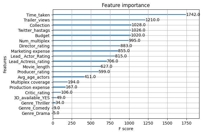
The xgb.plot_importance(xgb_clf) function is used to visualize the feature importance of an XGBoost model. It helps identify which features (input variables) have the most influence on the model's predictions.

xgb.plot_importance(xgb_clf)

#Grid search
xgb_clf = xgb.XGBClassifier(n_estimators=250, learning_rate=0.1, random_state=42)
param_test1={
    "max_depth": range(3,10,2),
    "gamma": [0.1, 0.2, 0.3],
    "subsample": [0.8, 0.9],
    "colsample_bytree": [0.8, 0.9],
    "reg_alpha": [1e-2, 0.1, 1]
}

grid_search = GridSearchCV(xgb_clf, param_test1, n_jobs=-1, cv=5, scoring='accuracy')
grid_search.fit(X_train, Y_train)
grid_search.best_params_
cvxg_clf = grid_search.best_estimator_
accuracy_score(Y_test, cvxg_clf.predict(X_test))

bestparams

{'colsample_bytree': 0.8, 'gamma': 0.1, 'max_depth': 5, 'reg_alpha': 0.01, 'subsample': 0.8}

Summary

Ensembling techniques combine multiple models to improve predictive performance and reduce overfitting. They leverage the strengths of individual models, aiming for better accuracy and robustness.

1. Bagging (Bootstrap Aggregating)

Involves training multiple models independently on different subsets of the data (generated through bootstrapping) and then aggregating their predictions (e.g., by averaging for regression or majority voting for classification).

Goal: Reduce variance and improve model stability.

Example: Decision Trees trained on various random samples.

2. Random Forest

An extension of bagging that specifically uses decision trees. It introduces randomness by selecting a random subset of features for each tree split, in addition to bootstrapping the data.

Goal: Improve accuracy and reduce overfitting by combining the predictions of many diverse trees.

Characteristics: Generally more accurate than a single decision tree and robust to noise.

3. Boosting

A sequential technique where each model is trained to correct the errors made by the previous models. Models are built one after another, with each new model focusing on the residuals (errors) of the prior ones.

Goal: Reduce both bias and variance, leading to a more accurate model.

Examples:

• AdaBoost: Adjusts the weights of misclassified observations to focus on harder-to-predict cases.

• Gradient Boosting: Fits new models to the residuals of previous models and typically involves a shrinkage parameter to control learning rate.

• XGBoost: An optimized version of gradient boosting that includes regularization to combat overfitting.

In machine learning, bias refers to the error introduced by simplifying the assumptions made by a model. A high bias means the model is too simple and may underfit the data, missing important patterns or relationships. Essentially, it's when the model fails to capture the underlying complexity of the data, leading to poor performance on both training and test data.

Happy Learning!