Merge Sort Explained: Step-by-Step Guide for Beginners

Previously, we explored Bubble Sort, Selection Sort, and Insertion Sort—basic sorting algorithms that help beginners understand sorting concepts. However, as we discussed, Bubble Sort struggles with large datasets, and both Selection and Insertion Sort have notable drawbacks due to their time complexity of O(n²), making them inefficient for larger datasets. Now, let’s dive into Merge Sort, a more efficient sorting algorithm with a time complexity of O(n log n). In this article, you will find a detailed explanation of Merge Sort and its algorithm, presented step-by-step with clear examples to make it easy for beginners to follow.

What is Merge Sort?

Merge Sort is a divide-and-conquer algorithm. It breaks a problem into smaller sub-problems, solves them independently, and combines the results. The core idea behind Merge Sort is to divide an array into halves, sort each half, and merge the sorted halves back together.

Unlike Bubble Sort, which repeatedly swaps adjacent elements, Merge Sort takes a more structured approach by dividing the array into manageable pieces and sorting those pieces before combining them.

How Merge Sort Works (Step-by-Step Breakdown)

Let's walk through an example to understand how Merge Sort works in practice.

Example:

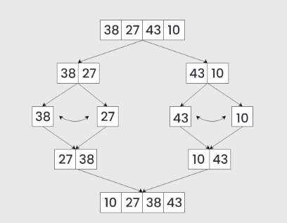
Imagine we have the following array to sort:

[38, 27, 43, 10]

Step 1: Divide the Array

The first step is to repeatedly divide the array into two halves until each sub-array contains only one element.

1. Initial Split:

   • Split [38, 27, 43, 10] into two halves:

       Left half: [38, 27]
       Right half: [43, 10]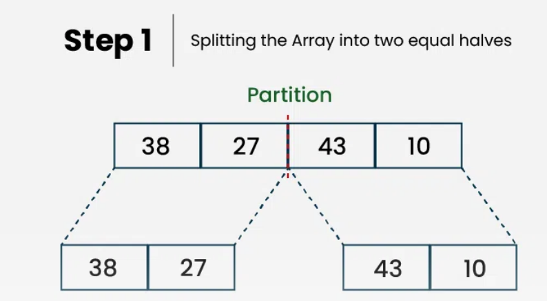
     

     

2. Further Split:

   • Split [38, 27] into:

       Left half: [38]
       Right half: [27]
     

   • Split [43, 10] into

       Left half: [43]
       Right half: [10]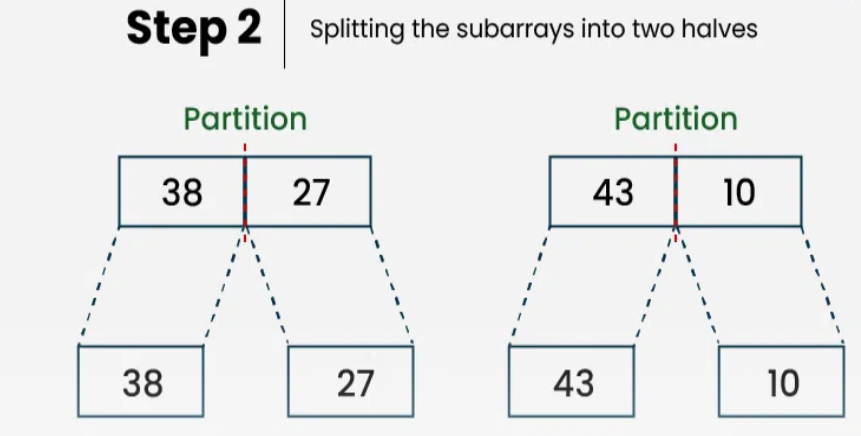
     

     

   • At this point, the array is broken down into individual elements:

       [38], [27], [43], [10]
     

Step 2: Merge the Sub-arrays

Now that we have single-element sub-arrays, we start merging them back together in sorted order.

1. Merging [38] and [27]:

   • Compare 38 with 27. Since 27 is smaller, it comes first.

   • The merged result is:

       [27, 38]
     

2. Merging [43] and [10]:

   • Compare 43 with 10. Since 10 is smaller, it comes first.

   • The merged result is:

       [10, 43]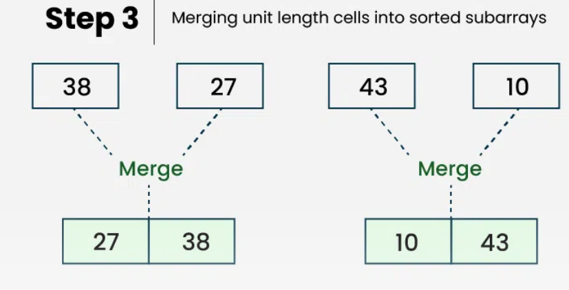
     

     

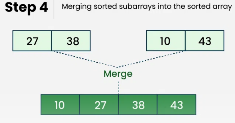
Step 3: Final Merge

Now we merge the two sorted halves [27, 38] and [10, 43]:

1. Compare 27 with 10. Since 10 is smaller, it comes first.

2. Compare 27 with 43. Since 27 is smaller, it comes next.

3. Compare 38 with 43. Since 38 is smaller, it comes next.

4. Finally, add 43 as it’s the last remaining element.

The final sorted array is:

[10, 27, 38, 43]

Pseudocode for the Merge Sort algorithm

Steps for Merge Sort:

1. Define the Function:

   • Create a function called mergeSort that takes an array as input.

2. Base Case:

   • Check if the length of the array is less than or equal to 1.

     • If true, return the array (it is already sorted)

3. Divide the Array:

   • Calculate the middle index of the array by dividing its length by 2.

   • Create two sub-arrays:

     • left_half contains elements from the start of the array to the middle index.

     • right_half contains elements from the middle index to the end of the array.

4. Recursively Sort:

   • Recursively call mergeSort on the left_half and store the sorted result in left_sorted.

   • Recursively call mergeSort on the right_half and store the sorted result in right_sorted.

5. Merge the Sorted Halves:

   • Create a function called merge that takes left_sorted and right_sorted as inputs.

   • Initialize an empty array called result.

   • Set two pointers, i and j, to 0 (for the left_sorted and right_sorted arrays, respectively).

6. Comparison and Merging:

   • While both pointers i and j are within the bounds of their respective arrays:

     • Compare left_sorted[i] and right_sorted[j].

     • If left_sorted[i] is less than or equal to right_sorted[j]:

       • Append left_sorted[i] to result.

       • Increment pointer i.

     • Otherwise:

       • Append right_sorted[j] to result.

       • Increment pointer j.

7. Add Remaining Elements:

   • After the comparison loop, if there are remaining elements in left_sorted, append them to result.

   • If there are remaining elements in right_sorted, append them to result.

8. Return the Merged Result:

   • Return the result array, which contains the merged and sorted elements.

Python Code for Merge Sort

Here’s how the Merge Sort algorithm is implemented in Python. This code follows the same steps we outlined above:

def merge_sort(arr):
    # Base case: if the array has 1 or 0 elements, it's already sorted
    if len(arr) <= 1:
        return arr

    # Find the middle point and divide the array into two halves
    mid = len(arr) // 2
    left_half = arr[:mid]
    right_half = arr[mid:]

    # Recursively sort both halves
    left_sorted = merge_sort(left_half)
    right_sorted = merge_sort(right_half)

    # Merge the sorted halves
    return merge(left_sorted, right_sorted)

def merge(left, right):
    sorted_array = []
    i = j = 0

    # Compare elements from both halves and merge them in sorted order
    while i < len(left) and j < len(right):
        if left[i] < right[j]:
            sorted_array.append(left[i])
            i += 1
        else:
            sorted_array.append(right[j])
            j += 1

    # If there are remaining elements in the left half, add them
    while i < len(left):
        sorted_array.append(left[i])
        i += 1

    # If there are remaining elements in the right half, add them
    while j < len(right):
        sorted_array.append(right[j])
        j += 1

    return sorted_array

# Example usage
arr = [38, 27, 43, 10]
sorted_arr = merge_sort(arr)
print(sorted_arr)  # Output: [10, 27, 38, 43]

Why is Merge Sort Efficient?

The key to Merge Sort's efficiency is its O(n log n) time complexity. This is due to the way it repeatedly divides the array in half (log n steps) and then merges each half back together in linear time (n steps). Unlike algorithms like Bubble Sort, which has a time complexity of O(n²) and becomes inefficient for larger datasets, Merge Sort ensures steady performance, even in worst-case scenarios.

Conclusion

In our previous discussions, we introduced the basics of sorting. Now, with Merge Sort, we've stepped into more advanced sorting techniques, gaining an understanding of how divide-and-conquer approaches can significantly improve efficiency. By breaking the array down into smaller parts, sorting them individually, and then merging them back together, Merge Sort provides a powerful tool for handling larger datasets.

Merge Sort is an important algorithm for both beginners and experienced developers alike. As you practice, you’ll find its methodical approach easy to understand and implement. Stay tuned for more insights on sorting algorithms and data structures as we continue this journey through the fundamentals of computer science!