What is an RNN Cell?

RNNs are great when you need to handle data that comes in a sequence, like text, sound, or time-series data. For example, to understand a sentence, you need to remember the previous words to make sense of the next one. RNNs are designed to do just that!

RNN Concepts

• RNN Cell: Keeps memory of past inputs, like remembering previous words in a sentence.

• Sequence Unrolling: The process of going step by step through data while keeping track of previous steps.

• Backpropagation Through Time: Going back to adjust past steps when the output isn’t correct, like practicing a song until you get it right.

• Gradient Accumulation: A technique for saving memory by accumulating updates (gradients) over multiple steps before applying them.

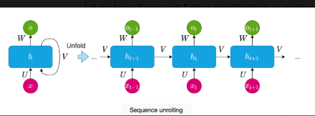
Sequence unrolling

This image shows the process of sequence unrolling in a Recurrent Neural Network (RNN). Imagine you’re reading a book. You don’t just look at one word; you also keep track of the previous words to understand the sentence. Similarly, an RNN processes each word (or data point) one at a time while "remembering" the previous ones. This is called sequence unrolling because the RNN looks at each part of the sequence (like words in a sentence) one by one, while keeping track of the past.

Here’s how it works:

1. Initial Input (x): The pink circles represent the input data (like words in a sentence). Let’s say x is the word you're hearing at a specific point in time.

2. Memory Block (h): The blue blocks represent the "memory" of the RNN. This memory is updated as each new word comes in. It keeps track of both the current word (x) and what it has heard before (from previous h).

3. Unrolling the Sequence:

   • First, the RNN processes the first word, stores some information, and then passes that information (along with the next word) to the next memory block.

   • This continues over time, with each memory block (h) updating based on the current word (x_t) and what it has already learned from the previous steps (like h_{t-1}).

   • This process is called unrolling because we take what was happening inside the RNN and stretch it out, step by step.

4. Outputs (o): The green circles represent the outputs, which are like the RNN’s understanding at each point. After processing each word (x_t), the RNN generates an output based on both the current word and the accumulated knowledge from previous words.

5. Connections (U, V, W): These arrows show the flow of information between the current input, the memory of previous steps, and the output:

   • U tells us how the current word (x) affects the memory.

   • V connects the memory (h) from one step to the next, ensuring that past knowledge is passed along.

   • W controls how the output is generated from the memory.

Backpropagation Through Time (BPTT)

Let’s say you’re learning how to play a song on the piano. You practice each note (step by step), but if you make a mistake, you need to go back and fix it. In RNNs, this process is called backpropagation through time. The RNN looks at each step (note) in the sequence, and if the output isn’t quite right, it goes back through time (previous steps) to adjust the connections, making sure it improves the next time.

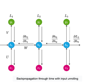
Let’s break down the components of the diagram:

1. Input (x): The pink circles (x1, x2, x3) represent the inputs at each time step. For example, each x_t could be a word in a sentence or a note in a song. The RNN processes these inputs one by one over time.

2. Hidden States (h): The blue circles (h1, h2, h3) represent the memory of the RNN at each step. Each hidden state (h_t) contains a summary of the current input and what has been learned from previous inputs.

3. Outputs (y): The green circles (y1, y2, y3) represent the outputs generated at each step based on the hidden states. Each output depends not only on the current input but also on the memory of previous steps.

4. Loss (L): The RNN calculates a loss (L1, L2, L3) at each step. Loss is like the model’s mistake or error — it’s a measure of how far off the predicted output is from the actual desired output.

Now, when the RNN finishes processing the sequence, it checks how well it did at each step (by calculating the loss L).

• If the output at time step 3 (y3) is wrong, the RNN doesn’t just correct the last step. It goes back in time, revisiting h2 and h1 to figure out how mistakes in earlier steps led to the final error.

• The partial derivatives shown in the diagram (∂h2/∂h1, ∂h3/∂h2, etc.) represent how the error (loss) from each time step is passed backward to adjust the earlier hidden states.

In other words, BPTT works by:

1. Calculating the loss at the final step (L3) and finding out how much the hidden state h3 contributed to that loss.

2. Moving backward through time, adjusting h2 and h1 based on their contribution to the overall error. This is done through the gradients (∂L/∂h), which tell the network how much to adjust at each step.

---

Analogy: Fixing a Mistake in a Song

Let’s say you’re playing a song and mess up on the last note. You don’t just practice the last note — you go back and play the whole section leading up to that note to see if you made a mistake earlier. The mistake might have started a few notes back, and fixing it early can prevent problems later.

That’s what BPTT does. It doesn’t just fix the mistake at the end; it goes back through all the steps to see where things went wrong, adjusting earlier steps to avoid repeating the same errors in the future.

Summary:

• The inputs (x1, x2, x3) are processed one by one, creating hidden states (h1, h2, h3).

• Each hidden state carries information from previous inputs.

• The model produces outputs (y1, y2, y3) and calculates errors (loss).

• Backpropagation Through Time allows the network to fix its mistakes by going back through the entire sequence and adjusting every step, not just the last one.

---

This code snippet shows a common technique used in deep learning training called gradient accumulation. Let’s break it down step by step.

Problem It Solves

When training large neural networks on machines with limited memory (such as GPUs), you may not be able to process large batches of data all at once. Gradient accumulation allows you to accumulate gradients over multiple smaller batches and then update the model’s weights as if you had processed a larger batch.

---

Key Concepts:

1. accumulate_gradient_steps = 2:
   This tells the model to accumulate gradients over 2 smaller batches before updating the model weights. Instead of updating the weights after each batch, the model waits until it has seen 2 batches.

2. for counter, data in enumerate(dataloader):
   Here, dataloader provides batches of data. The loop iterates over each batch, and counter is the index of the current batch.

3. inputs, targets = data:
   Each batch is split into inputs (e.g., images) and targets (e.g., labels). These are the data used to train the model.

4. predictions = model(inputs):
   The model processes the inputs and makes predictions based on its current knowledge.

5. loss = criterion(predictions, targets)/accumulate_gradient_steps:
   The loss function calculates the difference between the model's predictions and the actual targets. However, instead of using the entire loss from the batch, we divide it by accumulate_gradient_steps (2 in this case). This scales down the loss so that when it's accumulated over multiple batches, it behaves as if it’s calculated on a larger batch.

6. loss.backward():
   This is where the gradients are calculated. The gradients represent how much each parameter (weight) in the model needs to change to reduce the loss. However, at this point, the weights of the model are not updated yet — we are just collecting (accumulating) the gradients.

---

Accumulating and Updating the Gradients:

Imagine you’re baking cookies, but you can only bake a small batch at a time. Instead of cleaning the kitchen every time you make a small batch, you wait until you’ve made several batches and clean up all at once. This is the idea behind gradient accumulation. When training a neural network, if your computer (or GPU) doesn’t have enough memory, you don’t update the model right away. Instead, you calculate the updates (gradients) over several small batches, then apply all the updates at once. This helps save memory but still lets you learn efficiently.

if counter % accumulate_gradient_steps == 0:
    optimizer.step()
    optimizer.zero_grad()

1. if counter % accumulate_gradient_steps == 0:
   This checks if we have processed enough batches (in this case, 2 batches). When counter is a multiple of accumulate_gradient_steps (e.g., 2, 4, 6...), we update the model.

2. optimizer.step():
   This step updates the model’s weights based on the accumulated gradients. It’s like making the model smarter by adjusting the weights to reduce the loss.

3. optimizer.zero_grad():
   After updating the weights, we reset (zero) the gradients. This ensures that gradients from the next set of batches are accumulated from scratch, without interference from the previous accumulation.

---

Summary:

• You accumulate gradients over multiple small batches.

• After processing a set number of batches (2 in this case), you update the model’s weights.

• This technique helps when you don’t have enough memory to process a large batch all at once but still want the effect of a larger batch size.