Hey there! Welcome to Chapter 1 on Data Preprocessing!

Before getting into Machine Learning, let me tell you what you'll need:

• Educational requirement: Just some high school math, DSA (in python)

  (Probability and statistics will help you a lot. I have blog series on both DSA and statistics)

• IDE: Google Colab (TensorFlow, LightGBM, XGBoost, and all the powerful libraries for ML models are already installed in Google Colab).

• R is highly valued in machine learning because of its strong statistical foundation, rich libraries, and excellent visualization tools, which are essential for building and understanding ML models. However, if you have a basic PC or prefer to stick with Python, you don’t need to download R. We will start by learning and doing Data Preprocessing in Python

• CHATGPT: please use Ai if you stuck somewhere, it will help you a lot.

Introductory Part

The Machine Learning Process

There is typically a process to follow in ML -

1. Data Pre Processing

   • Import the data

   • Clean the data

   • Split into training and test sets

In this series, we don’t need to clean the data cause all of our data will be pre cleaned. We will hone on other important skills related to ML. But in real life, cleaning the data is quite important.

2. Modelling

   • Build the model

   • Train the model

   • Make prediction

This is a fun part of ML, here you will be dealing with several type of models.

3. Evaluation

   • Calculation performance metrics

   • Make a verdict

We will calculate if our proposed model is a fitting model or not. This is very important cause we need to be sure that the model we built serves the reason it was built for.

Splitting the data into a Training and Test set

Splitting the data into training and test set helps us to define how good our model works.

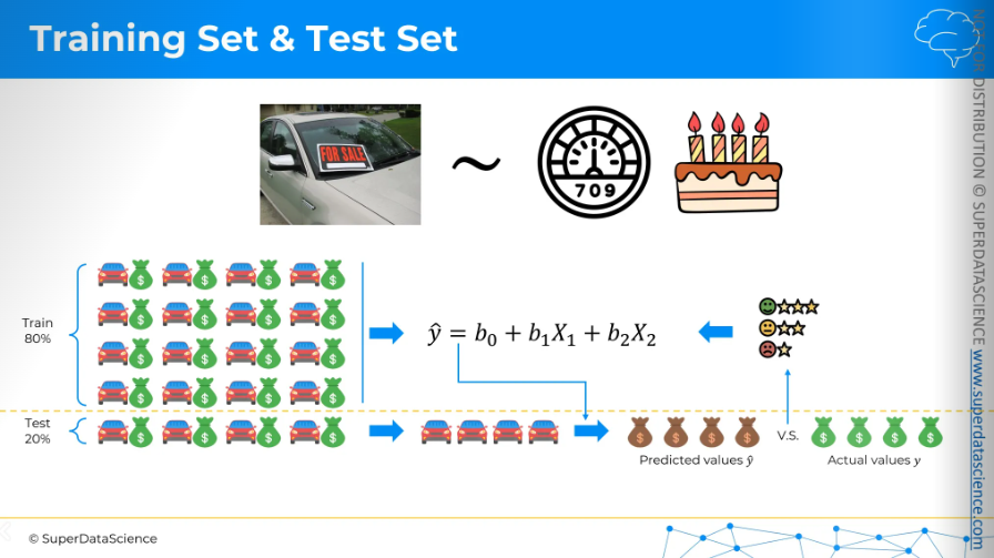
Imagine you need to predict car sale prices. This is your dependent variable. The independent variables are the car's mileage and age. You have data for 20 cars. Now, it’s time to split. Splitting data means setting aside a portion of your data before doing anything else. Usually, this is about 20% of your data, which will be your test set. The remaining 80% is your training set. We use the training set to build the model. After creating a linear regression model from the training set, we apply it to the cars in the test set. These cars weren't part of the model creation, right? (Think about it.) The model doesn't know anything about the 20% cars, so we use it to predict values and prices for the test cars.

The good news is that since we set aside this data earlier, we already know the real prices. Now, we can compare the predicted prices from our model, which hasn't seen these cars before, with the actual prices we know. This helps us evaluate our model. Is it working well? Is it not performing well? Do we need to make it better? That's how we split a training set and a test set, and why it's important to do so.

Feature Scaling

You always have to remember that feature scaling is always applied in columns, you would never apply it inside a row, okay?

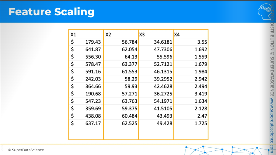
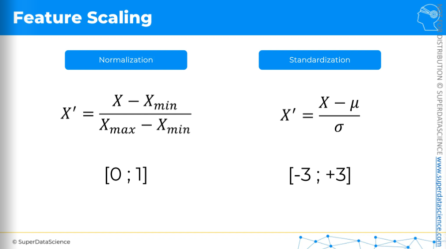
Now, let’s learn about feature scaling. There are multiple types of them, but here we’ll be focusing on two major types -

1. Normalization

   Taking the minimum value in a column, subtracting it from each value in the column, and then dividing by the difference between the maximum and minimum. Then you will end up wit a new column with values between 0 and 1.

   It is recommended when you have a normal distribution

2. Standardization

   Here we subtract the average, then we divide by the standard deviation. As a result, almost all the values of the new column will be between -3 to +3. If you have outliers or some extreme values, the result can go beyond this boundary.

   It actually works well all the time.

Here, a data set is given: annual income and age of a person. The task is to check which of the two people is more similar to the purple person.

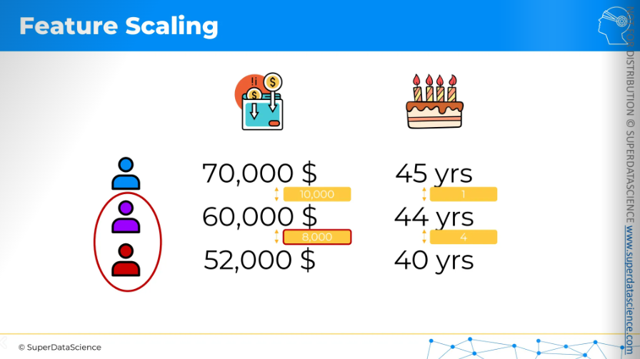
The two columns are not comparable because they relate to different things. Hence it’s important to scale your features. So let’s apply normalization to the columns one by one.

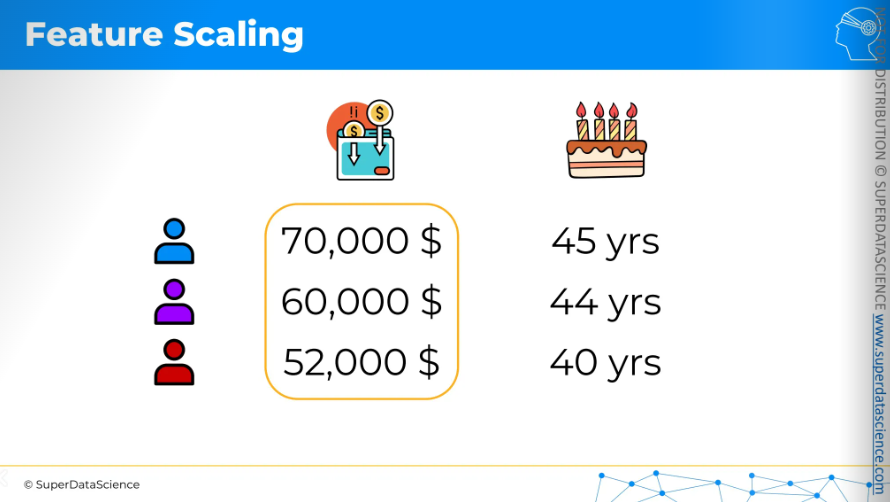
Once we apply our formula to the columns, the new values will look like this. Now, what do you think which person is closer to the purple person?

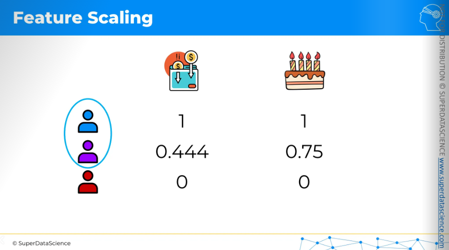
The answer is quite visible, blue person is closer to the purple person.

Data Preprocessing

Welcome to the very beginning of your Machine Learning journey. This is a very important part because whenever you build a ML model, you have to preprocess your data, right? You have to preprocess in the right way right? So that your model runs well on the data.

Now we’ll do some coding. I have uploaded a Colab file here. This is a read only file. So make a copy [file → Save a copy in drive] where you can edit as you like.

Colab file: https://colab.research.google.com/drive/1Dtn18VhKPQwJ4Bf0p23xtl2bm5ptMLx1?usp=sharing

Datasheet: https://drive.google.com/file/d/1cKxzNrnIMq4RxdMcBz3nlr7YtYaPhn5_/view?usp=sharing

After copying, what you are going to do is - delete all the code and keep just the texts. deleting the codes from copy file won’t be a problem as you have the original file.

After deleting, it should look something like this:

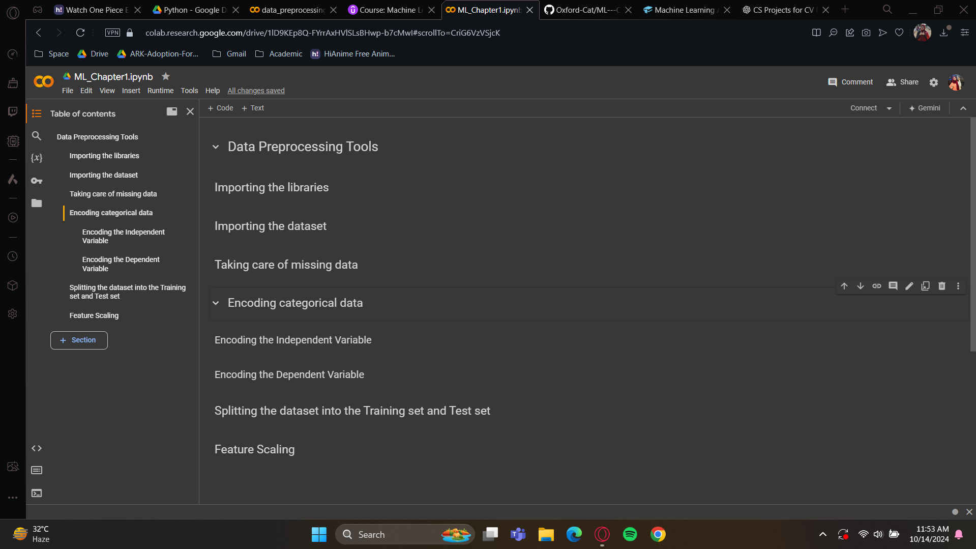
Here are the tools you will probably need for dataset preprocessing in your future ML models. So, it’s important for you to understand this implementation.

Data Preprocessing Tools

We are going to upload three libraries here -

1. NumPy: this will allow us to work with arrays.

2. matplotlib : it plots some nice charts.

3. pandas: it will help us to import dataset and create matrix of features and dependent variables.

Import syntax: import <name of the library> as <short name>

Do you know why we use short names? Because to use a module from the library (an ensemble of modules), we have to call it by the library name. To do it faster, we usually create a shortcut.

Import the dataset

To create the data frame, we'll use a function from the pandas library called read_csv(). We just need to enter the name of the dataset with its extension. (data set drive link is given)

Next, we'll create two things: one for the matrix of features and the other for the dependent variable vector.

Here's an important principle in machine learning: In any dataset used to train a model, you'll find features and the dependent variable vector. Can you guess what these are? Simply put, features are the columns used to predict the dependent variable. The dependent variable is the last column because the company wants to predict if future customers will buy a product based on this information. Features, or independent variables, contain the information used to make predictions. In any machine learning model, features are usually in the first columns, and the dependent variable is in the last column.

Creating x:

We have our dataset, right? To create x, we just need the first three columns. As mentioned, the last column is usually the dependent variable. We use the pandas function iloc, which stands for index location. This function extracts the indexes of the columns and rows we want. Start with the rows by using a colon [:] to indicate a range, meaning we take everything. In order to take everything excluding the last column, use :-1. That’s how we're setting our range from index zero up to index -1.

Creating y:

Alright, now let’s do the same for out dependent variable vector. First, we need to take our dataset to extract the last column. We use iloc to get the indexes of the rows and columns we want. We want all the rows because we need all the customers' purchase decisions, whether they bought the product or not. So, which column do we need? We only want the last column. What index do we use to get just the last column? Since we only need one column, we don't need a range. We'll use -1, which is the index for the last column. That's how we create the dependent variable vector. And that's it for this line of code.

[Using .values on a data-frame in Python converts it into a NumPy array, enabling faster computations and easier manipulation. Arrays are often preferred for machine learning tasks due to their efficiency and compatibility with certain algorithms.]

Now, to demonstrate how they work, we will print x and y. First, run the libraries. However, there's an important step to do before running the dataset: go to files and upload the dataset I have provided. Once Data.csv is uploaded, run the dataset cell.

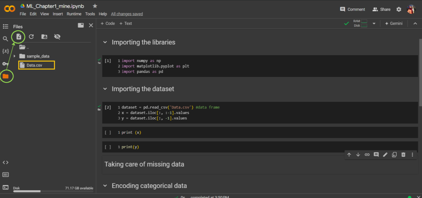
Now, run x and y, then open the dataset (double click on Data.csv) to check if they have been uploaded correctly.

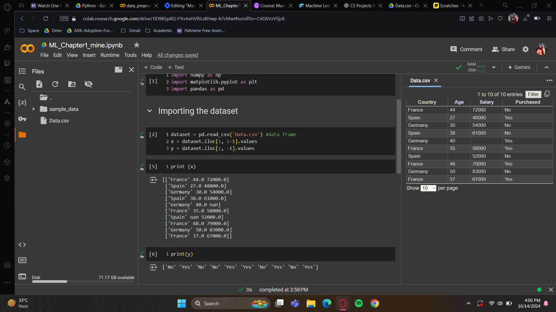
Have you gotten them correctly? Perfect! We now have our dataset, our matrix of features X, and our dependent variable vector Y. We created these because our future machine learning models going to need exactly these two inputs.

Summary of Object-Oriented Programming: classes & objects

A class is a blueprint for building something, like a house construction plan. An object is an instance of the class, like a house built from that plan. There can be many objects from one class, just as many houses can be built from one plan.

A method is a tool used on an object to perform an action, like opening the main door for a guest. It's a function applied to the object, taking inputs defined in the class and returning an output. Hope this helps.

Update: Simplified Indexing Explanation Added for Python beginners

I’ve added a section to explain indexing in regular Python lists, Pandas, and NumPy to make it easier for beginners. Here are the examples:

1. Regular python lists

   Python lists are ordered, and you can access elements by their index:

    my_list = [10, 20, 30, 40, 50]
    print(my_list[0])  # Output: 10
   
    # Access the last element using negative indexing
    print(my_list[-1])  # Output: 50
   
    # Slicing: Get elements from index 1 to 3
    print(my_list[1:4])  # Output: [20, 30, 40]
   

2. Pandas DataFrame index

   In Pandas, you often work with DataFrames. You can use .loc[] for label-based indexing and .iloc[] for position-based indexing:

    import pandas as pd
   
    # Create a simple DataFrame
    data = {'A': [1, 2, 3], 'B': [4, 5, 6]}
    df = pd.DataFrame(data)
   
    # Access the first row using `.loc[]` (label-based)
    print(df.loc[0])  
    # Output:
    # A    1
    # B    4
   
    # Access the first row and first column using `.iloc[]` (position-based)
    print(df.iloc[0, 0])  # Output: 1
   
    # Select the first two rows and columns using `.iloc[]`
    print(df.iloc[0:2, 0:2])  
    # Output:
    #    A  B
    # 0  1  4
    # 1  2  5
   

3. NumPy Array Indexing

   NumPy arrays allow for more advanced indexing techniques like multi-dimensional slicing:

    import numpy as np
    # Create a 2D array
    arr = np.array([[1, 2, 3], [4, 5, 6], [7, 8, 9]])
   
    # Access the element at row 1, column 2
    print(arr[1, 2])  # Output: 6
   
    # Slice the first two rows and columns
    print(arr[:2, :2])
    # Output:
    # [[1 2]
    #  [4 5]]
   
    # Select specific elements
    print(arr[[0, 1], [1, 2]])  # Output: [2, 6]
   

Taking care of missing data

You've probably noticed some missing data in your dataset. This doesn't always happen, but if it does, you need to address it, or it will affect your model.

There are a few ways to handle this. If your dataset is large, you can simply delete the missing data without affecting your results. That's one option.

However, you can't delete a lot of data, and if your dataset is small, you can't afford to remove any data. In such cases, you need to handle the missing data instead of ignoring it.

In the given datasheet example, there's a missing salary, we will replace it with the average of all the given salaries. This is the classic method for handling missing data, which I'll show you now.

To do this, we’ll need a library, and one of the best amazing library is scikit-learn. More than half of our models will use scikit-learn. To handle missing data, we’ll need the class SimpleImputer. The we will will create an object which will help us to put an average on the missing databox.

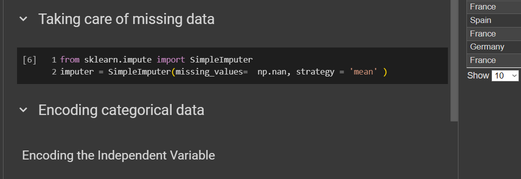
1. from sklearn.impute import SimpleImputer

   Since this is under scikit learn (known as sklearn), we have to import the library. SimpleImputer goes under impute so we have added that here.

2. imputer = SimpleImputer(missing_values = np.nan, strategy = ‘mean’)

   This is an object of the SimpleImputer class.

   missing_value - specifying what need to be replaced.

Now, remember this is just an object. We haven't connected it to our matrix of features yet. The next step is to apply this imputer object to the matrix of features.

The fit method connects the imputer to the matrix of features. It checks the missing values in the salary column and calculates the average salary. However, that's not enough for replacement. To replace the missing salary with the average, we need to call another method called transform, which applies the transformation. Let's do this.

This fit function needs all columns of X with numerical values, excluding text or categorical ones. The fit method will read the specified column. The first column contains strings, which might cause a warning or error. So, we'll only specify columns with numbers, like age and salary. I recommend selecting all numerical columns because, with large datasets, you won't easily spot missing values. Exclude string columns. This connects our imputer to the matrix of features.

Next, call the transform method from the imputer object to replace missing salaries and ages with their means. Input the same columns as in the fit method: age and salary. The transform method returns the updated matrix X with these replacements.

However, be careful, this transform method returns the updated matrix X with the replacements for the missing salary and age. So, take this second and third column of X matrix features and update it with the average age and salary returned by the transform function of the imputer object.

Let’s print and check.

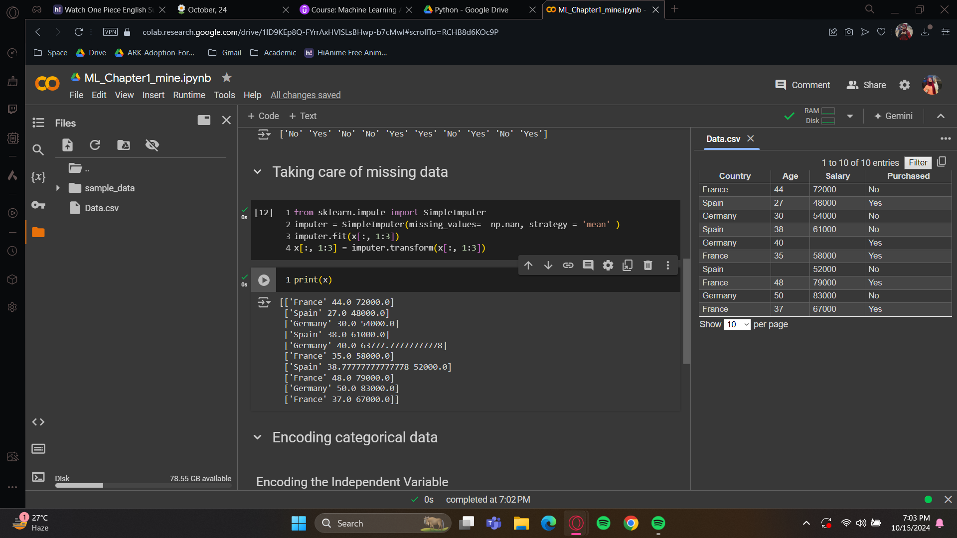
The missing data has been updated with the mean. Congratulations! Now you have another tool in your data processing toolkit.

Encoding categorical data

Encoding the Independent Variable

The country column and purchased column has strings in them. Our machines can’t read the strings values, and we have to work with non-numerical data too. If we don’t handle them, our model will be a faulty model. Hence, we have to encode our categorical data.

1. Import Libraries:

   • ColumnTransformer from sklearn.compose: This allows us to apply different preprocessing steps to specific columns of the data.

   • OneHotEncoder from sklearn.preprocessing: Used to convert categorical features into a one-hot encoded format.

2. Define ColumnTransformer:

   • ct = ColumnTransformer(...): A ColumnTransformer is initialized with a transformer that specifies how to transform certain columns.

     • transformers: A list of tuples specifying which transformations to apply.

     • ('encoder', OneHotEncoder(), [0]): This means we are applying a OneHotEncoder to the first column (index [0]) of the data.

     • remainder='passthrough': This tells the transformer to keep all other columns unchanged (i.e., pass through).

3. Fit and Transform:

   • ct.fit_transform(x): This applies the transformation (in this case, one-hot encoding) to the dataset x. It fits the transformer to the data and returns the transformed version.

   • np.array(...): Converts the result into a Numpy array.

Important Key Elements:

• OneHotEncoder: Converts categorical variables into a format that can be provided to machine learning algorithms by encoding each category as a binary (0/1) variable.

• ColumnTransformer: Allows you to apply different preprocessing to different columns in a dataset.

• remainder='passthrough': Keeps any columns that were not transformed in their original form.

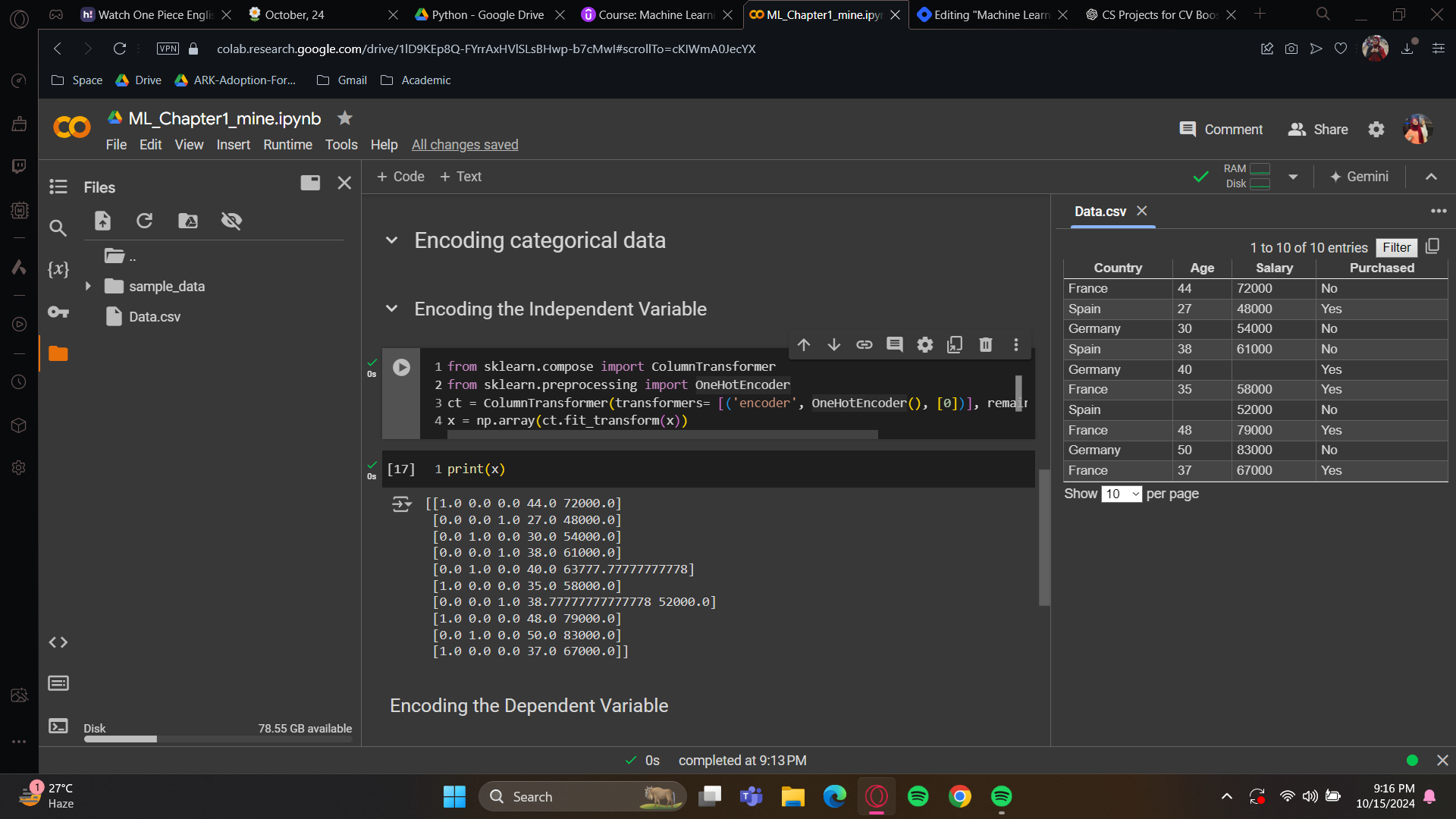
As you can see, France turned into 1.0 0.0 0.0, Spain turned into 0.0 0.0 1.0 just as we wanted.

Encoding the Dependent Variable

For the last column, it is indeed in text format. And we would like to turn the yes/no into 1/0 format. To do this, we will import another class which will turn them into binary format.

Again, import LabelEncoder from sklearn.preprocessing. Place the class into a variable. The good news is, it has builtin transformer so no need for extra hassle with transforming.

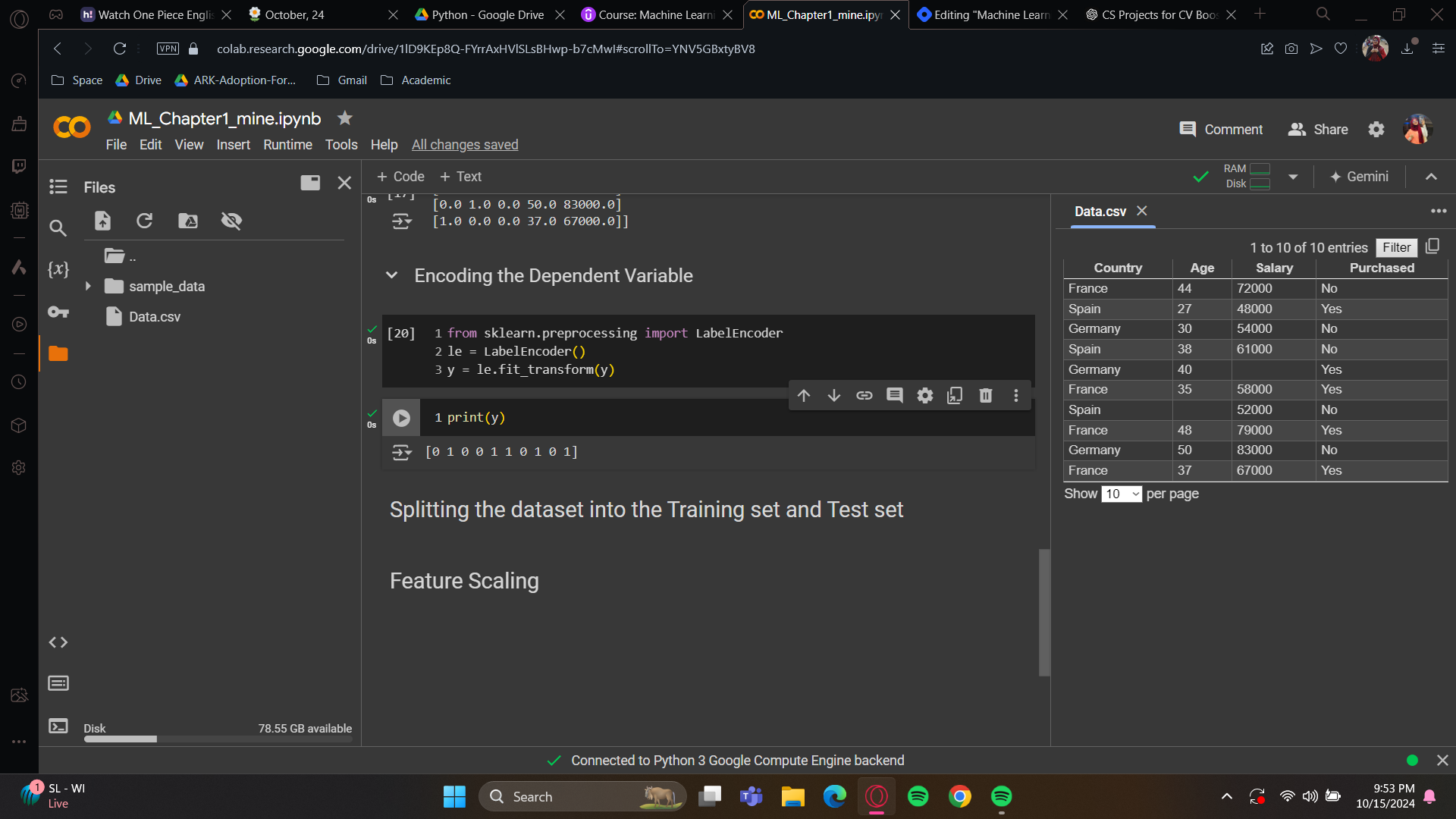
Now you know how to apply one-hot encoding when you have several categories in a feature of your feature matrix. You can also use simple label encoding when you have two classes that can be directly encoded into zeros and ones, resulting in a binary outcome. All right, perfect.

Splitting the dataset into the Training set and Test set

Before we begin, I want to address a common question in the data science community: Should we apply feature scaling before or after splitting the dataset into the training and test sets? I've seen this question asked many times in various data science forums. Some people say to scale before the split, while others say to do it after. There is only one correct answer: we should apply feature scaling after splitting the dataset into the training and test sets.

Why? In real-world scenarios, the model will only have access to the training data, so the scaling should be done based solely on the training set. The test set should be treated as unseen data, so you should scale it using the same parameters (mean, standard deviation, etc.) computed from the training data. By splitting first, the scaling is applied independently to the training set and then those scaling parameters are used to transform the test set. This ensures a more accurate and realistic evaluation of the model’s performance as well as avoiding information leakage.

All right, so I think I've explained enough!!

All right, how are we going to do this?

We'll use a function from scikit-learn, the popular data science library. It has a module called model_selection, which includes a function named train_test_split. And this function will exactly do what we want, which is to create four separate sets, not just two, but four, because we will create a pair of feature matrices and dependent variables for the training set, and another pair of feature matrices and dependent variables for the test set.

• X train: the matrix of features of the training set

• X test: the matrix of features of the test set

• Y train: the dependent variable of the training set

• Y test: the dependent variable of the test set

Actually, this isn't our requirement; it's what the machine learning model needs—four sets. This format is expected by our future machine learning model.

It’s obvious that the train_test_split will have 4 arguments. First, the matrix of features, then the dependent variable vector, then the test size (I recommend having 80% of observations in the training set and 20% in the test set). Finally, as the observations will be randomly split into the training and test sets, we'll set random_state = 1 to ensure consistency.

Alright now for the trust reveal: Let’s run these cells

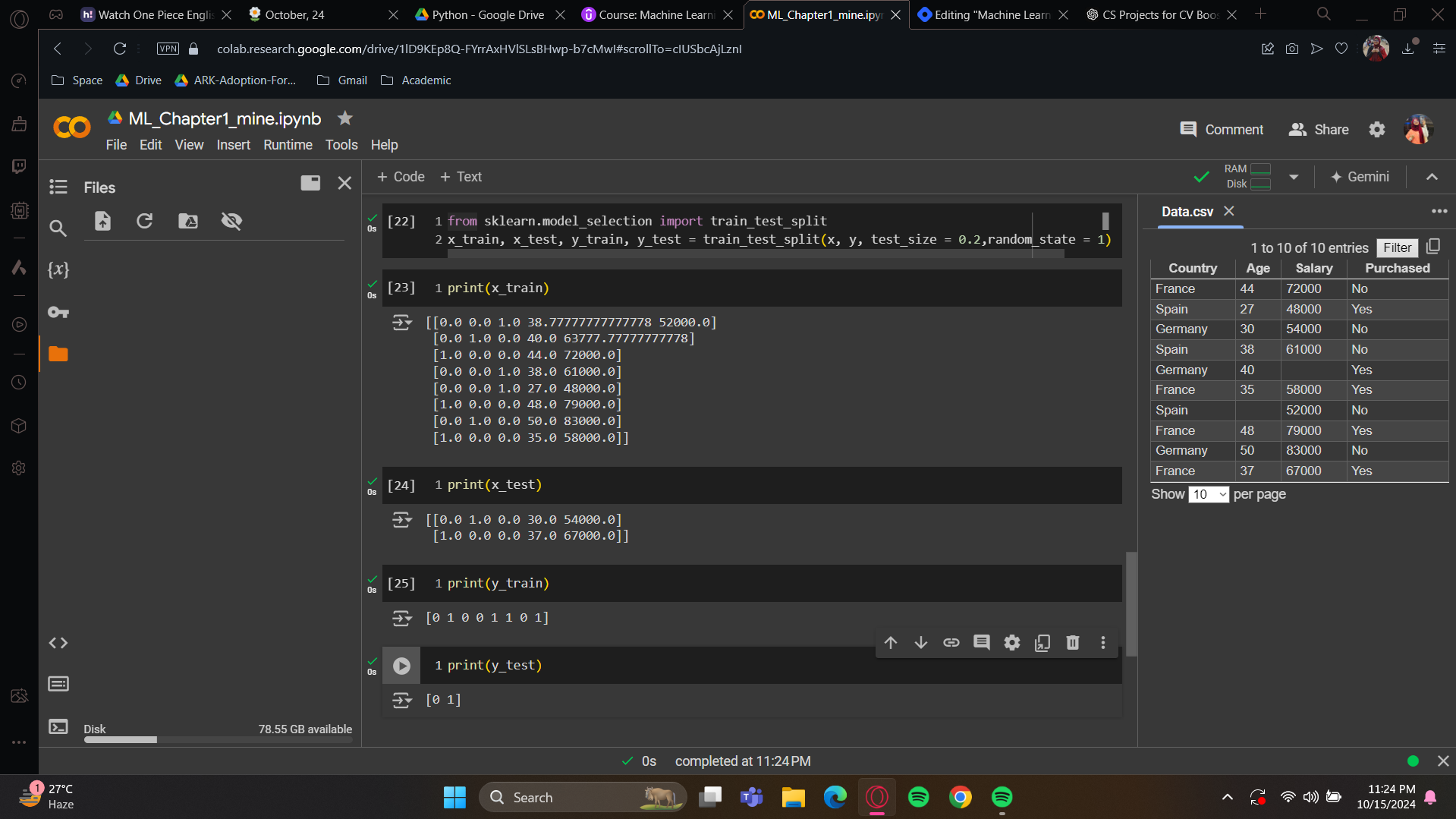
1. x_train: We now have 8 observations in the training set. These are eight randomly selected customers from the dataset. The first three columns are the one-hot encoded variables for the country category, also known as dummy variables.

2. x_test: We’ll get two observations here.

3. y_train: we got 8 purchased decisions right? Please note that these 8 decisions are corresponded with the 8 observations of the x_train set. These are the same customers here.

4. y_test: 2 purchase decisions, zero and one, corresponding to the same customers as in the test set matrix of features.

Now, let's move on to our final tool: feature scaling. As you know, this should be applied right after the split. You'll see the results with some prints after we apply this to our dataset.

Feature scaling

Before starting, let me tell you that feature scaling isn't needed for all machine learning models, only some. For many models, we don't need to apply feature scaling, even if features have very different values.

We'll use a class called StandardScaler to standardize both the feature matrix of the training set and the feature matrix of the test set. You don’t need to apply feature scaling to the dummy variables. The goal of standardization in feature scaling is to bring all feature values into the same range. Since our dummy variables already have values in the range of [-3, +3], there's nothing to be done with them. Moreover, applying standardization would make it worse because it would transform these values again between -3 to +3, causing us to lose our interpretation. So don’t do this. Only apply feature scaling to your numerical values.

As i told, we are going to apply scaler on training set only. So here, i’m taking the x_train set. Remember the trick to take all the rows, which is put a colon :. As for the columns, we have to take care of - the index of the age is 3. Then put a colon. So this will take everything from index to to the last one (which in this case in salary). Last column is not going to be added

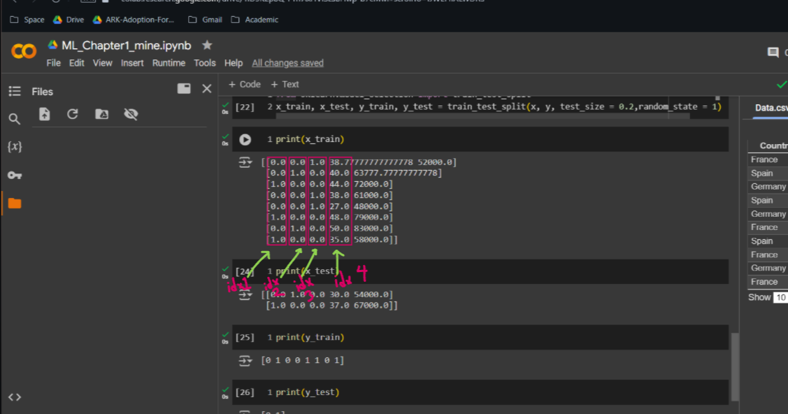
Now for the print:

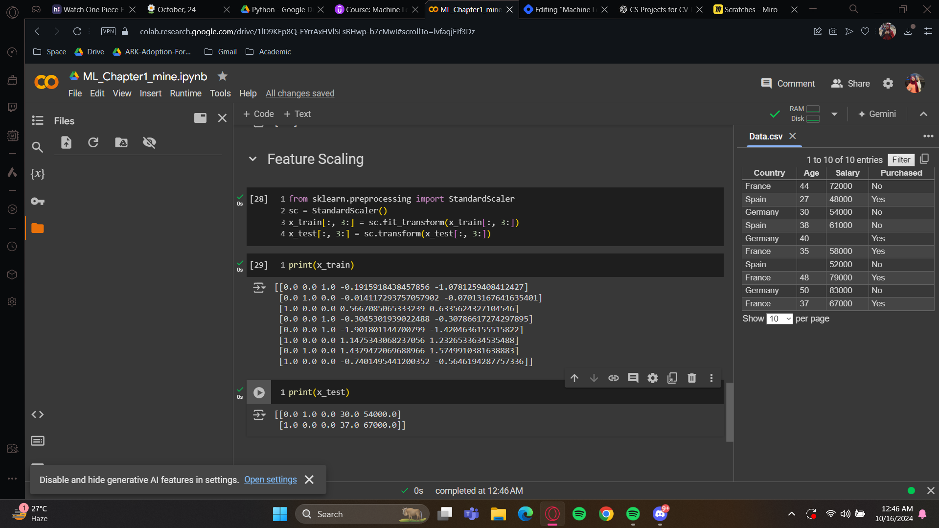
As you can see, the age and salary is showing updated values. These are between -3 to +3 so all of them falls under a range. And for the x_test, well, you still have your dummy variables for the same two customers, but the age and salary are scaled to values between minus two and plus two.

Data preprocessing template

This is the template we will always need to build a model. I’m sharing this to you as you have successfully gone through the whole blog. Congratulations!

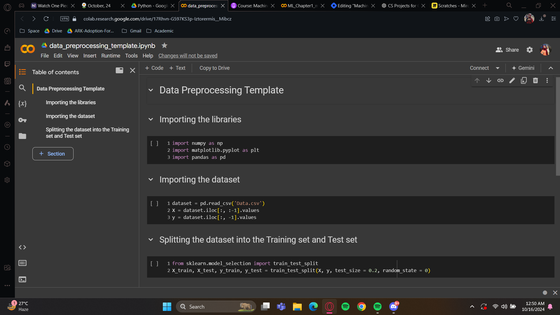
Make sure to have this template ready each time we build our future machine learning models.

Now, take a good break, you deserve this after completing this data preprocessing phase. Take your time to understand everything, and once you're ready to start with the first part of machine learning, which is regression, let's continue our journey together in the next section.