Welcome to Part 2 - Regression!

Regression models (both linear and non-linear) are used for predicting a real value, like salary for example. If your independent variable is time, then you are forecasting future values, otherwise your model is predicting present but unknown values.

In this chapter, you will understand and learn how to implement the following Machine Learning Regression models:

2.1 Simple Linear Regression

2.2 Multiple Linear Regression

2.3 Polynomial Regression

2.4 Support Vector for Regression (SVR)

2.5 Decision Tree Regression

2.6 Random Forest Regression

Simple Linear Regression Intuition

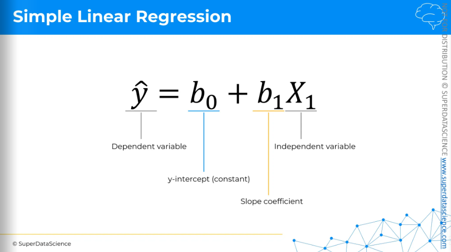
On the left, we have our dependent variable which we want to predict. On the right, we have our independent variable which is our predictor.

Using this equation, we are going to predict the out put of potatoes in a farm based on the amount of fertilizer used.

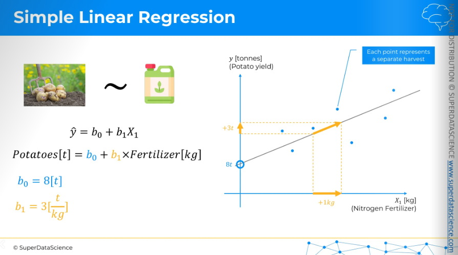
The slope coefficient indicates that potato harvest increases by 3 tons for every 1kg fertilizer. So that’s how linear regression works. [The numbers are all made up for illustrative purpose]

Ordinary Least Squares

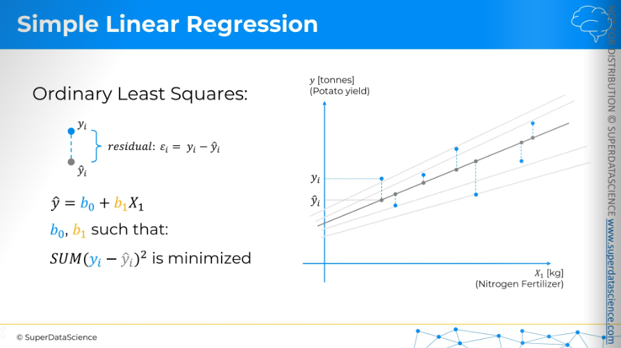
The question is, which of the slope line is the best suitable line for our slope. There can be and there indeed are multiple candidates as we can see. To define the best fit, what we have to do is apply ordinary least sq. method. (Visually) take a data point of a slope line and project them vertically on our linear regression line. For the sake of simplicity, we are doing it only with the middle one here. But keep in mind that we have to do this for each of the slope lines, okay?

We have our yi and yi^ here. The difference between them is called residuals. The best equation is where the b0 and b1 are such that the sum of the squares of the residual is minimum. That’s why it’s called the ordinary least sq. method. So for whichever regression line we find the smallest value is going to be out best fit.

Simple Linear Regression Steps

Resources:

1. Colab file: https://colab.research.google.com/drive/1FTA1PEwJX-omLT3WitBHjFEn17S6BCpZ (make a copy for yourself)

2. Datasheet: https://drive.google.com/file/d/19NyGm-zJLtKKDNt8Mkr99-ZxY8RaUZKF/view (download it)

3. Data preprocessing template: https://colab.research.google.com/drive/17Rhvn-G597KS3p-Iztorermis__Mibcz

As you have done it before, upload the datasheet in your copy file.

Let’s start building our first machine learning model which will generate some linear values!

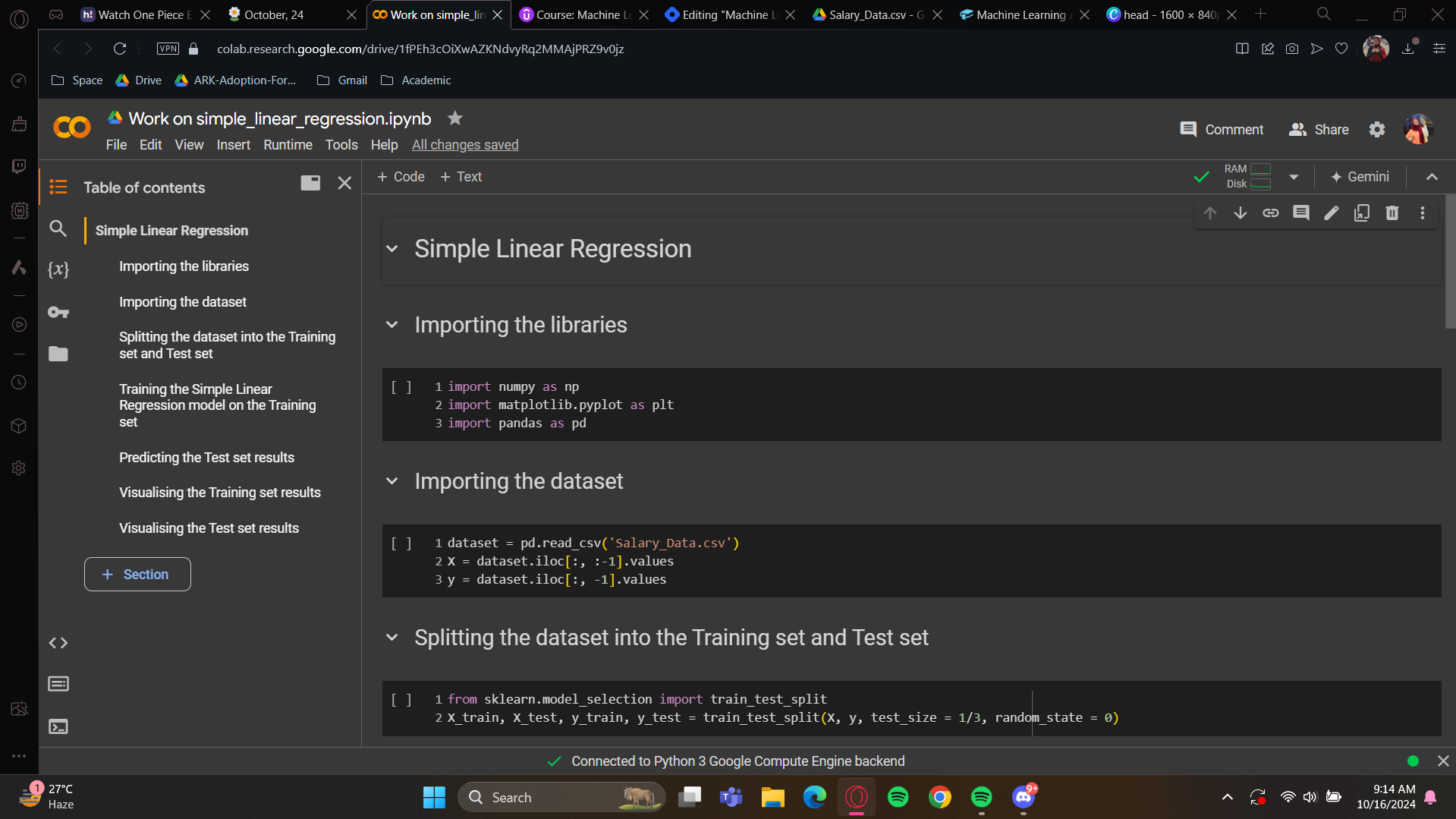
If you go to the contents, you’ll see the template is given there already. Now, delete all the code cells so that we can hands-on build them one by one.

I hope you are ready now. Our first step is obviously data preprocessing and maybe implement of some tools so that our future linear regression model can be trained on the data set. Now simply copy and paste from the given data preprocessing template.

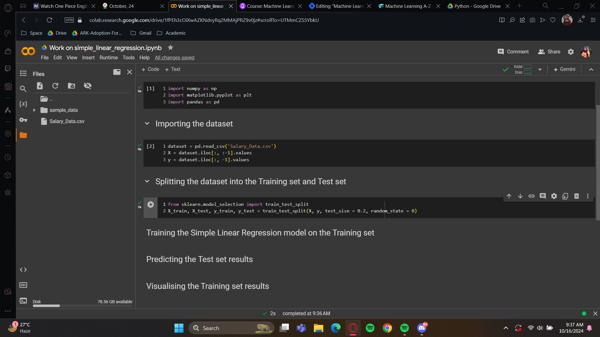
Now it should look something like this, except for the name of the data sheet. After that, upload the downloaded datasheet. Now execute the cells, and voila! Your data preprocessing is complete!

Okay! Time to focus on the linear regression model. So for that, we have to import some classes. Or we can build from scratch. But i’m going to provide you a very clear template, which will allow you to make a linear regression model in the simplest way so we are not going to build from scratch, i hope that’s fine with you.

It’s very simple right? These 2 line of codes directly creates the linear regression building model!

But now, of course, we need to train it using the training set, therefor we have to link it to the training set. And the function that connects it for training is the fit function.

The fit method will train the model, also it expects the x and y train set in it.

Congratulations! You have created your very first machine learning model! I’m so happy for you! But this is just the beginning. Gradually we’ll move on to more complex machine learning models. And this is the reason i’m providing you templates in order to do it as efficiently as possible.

Now it’s time to move onto the prediction. We split this dataset into a training set and a test set. The test size was set to 0.2, which means 20% of the observations went into the test set. So, 20% of 30 is six. Now, we will input the number of years of experience for each of these six employees into the predict method. Our model will then predict their salaries. We will compare our predicted salary with the real salaries.

Here, we only need the years of experience to predict salaries. These are in X test, which contains the experience data for the test set. So, we just input X test. I would like to keep the all predicted value in a new variable.

Moving to the next, Now we want to create a nice graphic to show the real salaries compared to the predicted salaries. Essentially, we'll have a 2D plot.

plt.plot(X_train, regressor.predict(X_train), color = ‘blue) :This code visualizes the regression line learned during training, showing how well the model fits the data.

• plt.plot(): Creates a 2D line plot.

• X_train: The training data used for the model.

• regressor.predict(X_train): The model's predictions based on X_train.

• Plotting the regression line: Plots X_train against regressor.predict(X_train) to show the predicted line.

• color = 'blue': Colors the line blue.

For the visualization of test set, we will just copy and paste the code changing the co-ordinate names.

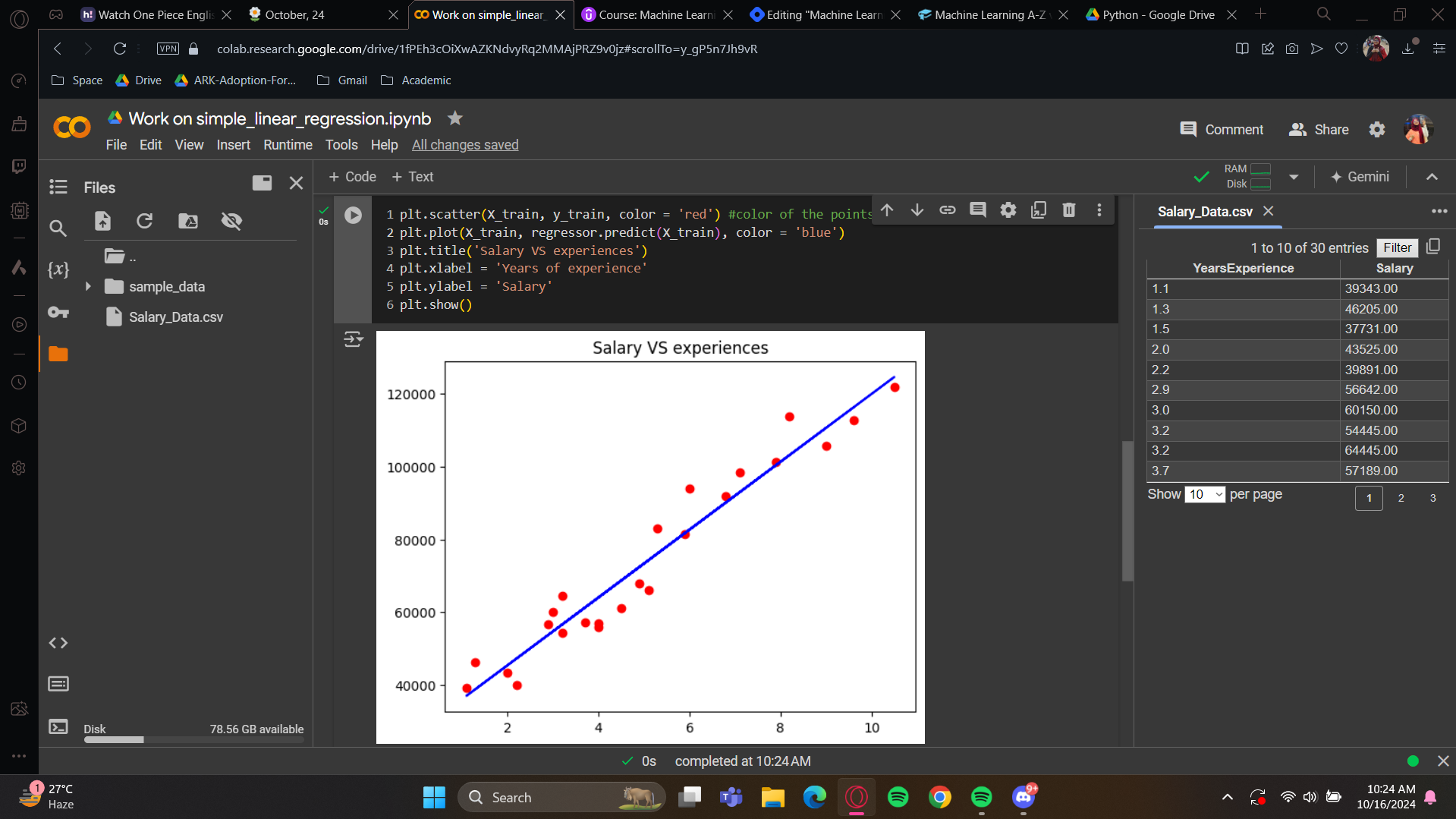
Let's see if we're still close to the real salaries, even for new observations.

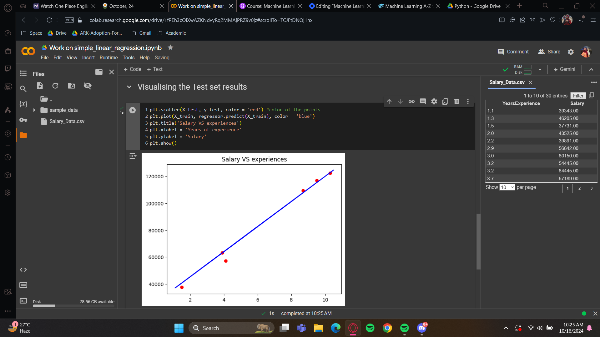
See how we are getting two beautiful graphs? Yes, our predicted salaries, shown on the blue line, are very close to the real salaries. Our simple linear regression model did a great job predicting new observations.