Major League Baseball is the second richest sports league in the world, generating more than $11 billion in annual revenue. It also has boasts the highest fan attendance per season among all leagues. Given this financial scale, baseball analytics has become a critical field, with its roots dating back over a century. Though it experienced a significant leap in analytical methods during the “Moneyball” era of the early 2000s.

This post explores a statistical method known state space modelling, applying it to analyse sports team performance.

In this analysis, I’ve implemented a state space model using Bayesian inference to assess MLB team performance throughout the 2022 season.

The dataset used is a comprehensive collection of final scores from MLB games spanning multiple seasons.

Modeling Team Performance with State Space Models

A State Space Model (SSM) is a powerful framework used to model time-series data, capturing the evolving state of a system over time. In the context of sports, the system we care about is the underlying "strength" or "performance" of a team, which we cannot directly observe but can infer from outcomes like game scores.

In finance, these models are used to estimate hidden variables like market volatility or economic indicators based on observed data such as stock prices. Similarly, in baseball, team performance can be thought of as a latent (hidden) state that evolves game by game, influenced by factors like player health, form, strategy changes, and other external inputs.

The Model

For this project, I used a Bayesian State Space Model to identify the latent team rating across the 2022 MLB season. State space models consist of: the state equation and the observation equation.

State Equation:

The state equation defines the evolution of a team’s rating over the season. For simplicity, we can assume that each team’s rating follows a random walk, where their rating at game $t$ depends only upon their rating at the previous game $t-1$ plus some random noise.

$$x_t = x_{t-1} + w_t$$

Here, $x_t$ represents the latent rating of the team at game $t$, with $w\_t$ representing the process noise; the random fluctuations in team performance between games. This “noise” could be reflecting factors such as: injuries, player transfers, tactical changes etc.

Observation Equation:

The observation equation connects the latent team ratings to the observed game outcomes - in this case, the score difference between the two teams in each game. The observed score difference depends on the difference in the latent ratings of the two teams:

$$y_t = x_t^{(team1)} - x_t^{(team2)} + v_t$$

Here, $y_t$ is the observed score difference in game $ t $ , with $v_t$ being the observation noise, accounting for randomness in the game (e.g., weather, referee decisions, bad luck etc.).

Data Preprocessing

Before applying the state space model, we need to preprocess the data.

import pandas as pd

# Load the data
df = pd.read_csv('mlb_elo.csv')

# Convert date column to datetime
df['date'] = pd.to_datetime(df['date'])

# Filter for the 2022 season
df = df[df['season'] == 2022]

# Prepare observed scores for Bayesian modelling
df['score_diff'] = df['score1'] - df['score2']  # Score difference (Team 1 - Team 2)

# Create the flipped version of the dataframe where home and away are swapped
df_flipped = df.copy()
df_flipped['team1'], df_flipped['team2'] = df['team2'], df['team1']  # Swap teams
df_flipped['score_diff'] = -df['score_diff']  # Reverse score difference

# Combine the original and flipped dataframes
df_combined = pd.concat([df, df_flipped], ignore_index=True)

# Sort by date to keep chronological order
df_combined = df_combined.sort_values('date').reset_index(drop=True)

Mapping Teams

We then map each team’s name to a unique index to refer to teams numerically in the model. The game indices are also prepared to track each team’s games in chronological order.

# Map team names to indices for the Bayesian model
teams = sorted(set(df_combined['team1']).union(set(df_combined['team2'])))
team_to_idx = {team: idx for idx, team in enumerate(teams)}

team1_idx = df_combined['team1'].map(team_to_idx).values
team2_idx = df_combined['team2'].map(team_to_idx).values

# Prepare game indices for both teams
df_combined['team1_game_idx'] = df_combined.groupby('team1').cumcount()
df_combined['team2_game_idx'] = df_combined.groupby('team2').cumcount()

# Make sure max games played covers both home and away games
team_game_counts = df['team1'].value_counts() + df['team2'].value_counts()
max_games_played = team_game_counts.max()

# Create arrays of game indices for each team's games (home and away combined)
team1_games = df_combined['team1_game_idx'].values
team2_games = df_combined['team2_game_idx'].values

# Prepare observed scores (for both original and flipped games)
observed_scores = df_combined['score_diff'].values

Bayesian Inference

To estimate the latent team ratings, I employed Bayesian inference, which allows us to incorporate prior beliefs about the teams' strengths (based on historical performance, for example) and update those beliefs as more data (games) become available. By using Bayesian methods, we not only obtain point estimates of the team ratings but also quantify the uncertainty around those estimates.

In the model, we placed a Gaussian prior on the initial team ratings, with a small variance indicating our initial uncertainty about the teams' performance at the beginning of the season. The random walk variance was also estimated from the data, reflecting how much teams' performances fluctuate from game to game.

Below is the code that implements this, using PyMC, a Python library for Bayesian modelling.

import pymc as pm

with pm.Model() as state_space_model:
    # Prior for initial team ratings at the beginning of the season
    mu = pm.Normal('mu', mu=0.001, sigma=0.5)  # Overall team rating prior
    sigma_team = pm.HalfNormal('sigma_team', sigma=0.8)  # Prior for random walk process variance

    # Latent team ratings, one for each team across all games
    team_ratings = pm.GaussianRandomWalk('team_ratings', sigma=sigma_team, 
                                         shape=(len(teams), max_games_played), 
                                         init_dist=pm.Normal.dist(mu=mu, sigma=sigma_team))

    # Score differences depend on the evolving ratings of team1 and team2 for each game
    scores = pm.Normal('scores',
                       mu=team_ratings[team1_idx, team1_games] - team_ratings[team2_idx, team2_games],
                       sigma=4,  # Observation noise
                       observed=observed_scores)

    # Sample from the posterior
    trace = pm.sample(1000, tune=2000, target_accept=0.97)

Sampling the Posterior Distribution

In the code above:

The team ratings are modeled using a GaussianRandomWalk, which captures how each team's strength evolves throughout the season.
The score differences between teams are modeled as a normal distribution, with the mean being the difference between the latent ratings of the two teams in each game.
Finally, we use MCMC sampling (pm.sample) to sample from the posterior distribution. This process allows us to estimate the parameters of interest (team ratings over time) and quantify the uncertainty around these estimates.

By sampling 1000 posterior samples (after a tuning phase of 2000 iterations), we can analyze how each team's performance changes game by game, and see how certain or uncertain we are about those estimates.

# Extract team ratings over time from the InferenceData object
team_ratings_samples = trace.posterior['team_ratings'].values

# Calculate the mean team ratings over time
mean_team_ratings_over_time = team_ratings_samples.mean(axis=(0, 1))  # Averaging over chains and samples
# List of teams of interest
teams_of_interest = ['LAD', 'ANA', 'NYM', 'SDP', 'PIT', 'OAK']  # Feel free to change to any teams of interest

plt.figure(figsize=(12, 6))

# Plot rating evolution for each team in the list
for team in teams_of_interest:
    team_idx_of_interest = team_to_idx[team]

    # Find the number of games this team played
    games_played_by_team = df[(df['team1'] == team) | (df['team2'] == team)].shape[0]

    # Plot the mean team ratings over the games the team played
    plt.plot(mean_team_ratings_over_time[team_idx_of_interest, :games_played_by_team], label=team)

# Customize the plot
plt.xlabel('Game Index')
plt.ylabel('Mean Team Rating')
plt.title(f'Mean Team Ratings for {", ".join(teams_of_interest)} Over the Season (2022)')
plt.legend()
plt.show()

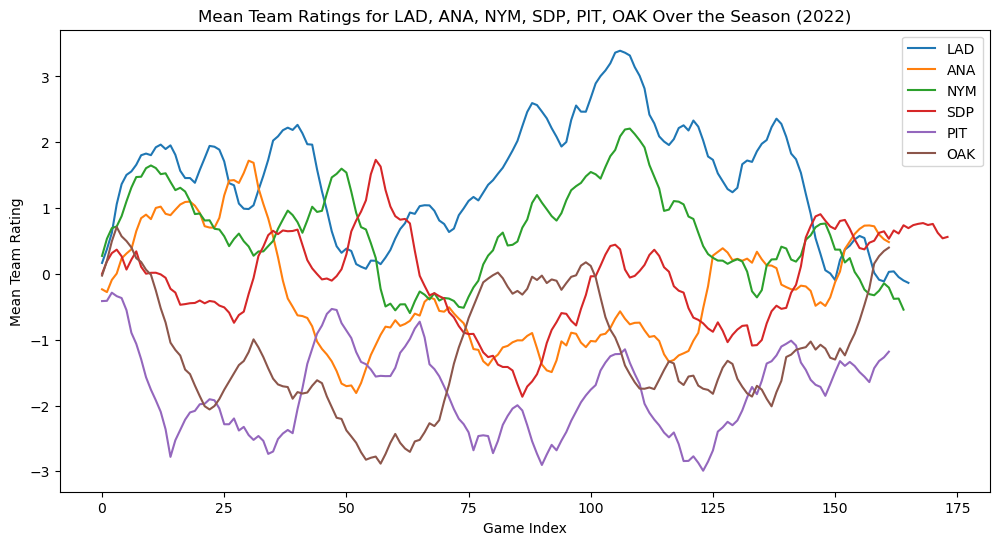
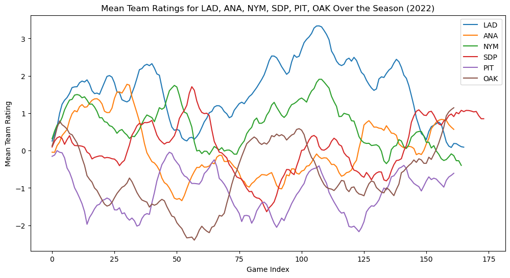
This produces a state space model for the performance of various teams across a season. But can we improve this model?

The model currently is simple enough, but the original dataset, provides a rating of both starting pitchers. We can include this as a term, alongside a home/away indicator, to give us a more accurate rating.

Our state equation remains the same, but our observation equation will now change to reflect these additional factors:

$$y_t = (x_t^{team\space1} - x_t^{team\space2}) + \beta_{home} \cdot h_t + \gamma \cdot (p_{t_1} - p_{t_2}) + v_t$$

Where:

$x_t^{team\space1}$ and $x_t^{team\space2}$ are the latent strengths (ratings) of the two teams.
$\beta_{home}$ is the coefficient representing the influence of the home/away advantage.
$h_t$ is the home indicator, which is 1 if team 1 is playing at home and -1 if they are playing away.
$\gamma$ is the coefficient representing the influence of the pitcher rating.
$p_{t_1}$ and $p_{t_2}$ are the pitcher ratings for team 1 and team 2, respectively.
$v_t$ is the observation noise.

Interpretation:

The team rating difference $(x_t^{team\space1} - x_t^{team\space2})$ is still the core of the model.
The home/away advantage $\beta_{home} \cdot h_t$ adjusts for whether team 1 is playing at home or away.
The pitcher influence $\gamma \cdot (\space p_{t_1}-p_{t_2})$ adjusts the score difference based on the relative pitcher ratings.

with pm.Model() as state_space_model:
    # Priors for team ratings
    mu = pm.Normal('mu', mu=0.001, sigma=0.5)
    sigma_team = pm.HalfNormal('sigma_team', sigma=0.8)

    # Home advantage prior
    home_advantage = pm.Normal('home_advantage', mu=0.0, sigma=1.0)

    # Pitcher influence rate prior (how much the pitcher's Elo affects the score)
    pitcher_influence = pm.Normal('pitcher_influence', mu=1.0, sigma=0.5)

    # Latent team ratings
    team_ratings = pm.GaussianRandomWalk('team_ratings', sigma=sigma_team, 
                                         shape=(len(teams), max_games_played),
                                         init_dist=pm.Normal.dist(mu=mu, sigma=sigma_team))

    # Score differences depend on team ratings, pitcher Elo with influence factor, and home advantage
    scores = pm.Normal('scores',
                       mu=(team_ratings[team1_idx, team1_games] - team_ratings[team2_idx, team2_games]
                           + pitcher_influence * (pitcher1_rgs - pitcher2_rgs)  # Pitcher Elo with influence
                           + home_advantage * home_indicator),
                       sigma=4,  # Observation noise
                       observed=observed_scores)

    # Sample from the posterior
    trace = pm.sample(1000, tune=2000, target_accept=0.97)

Limitations

Despite the statistical insights, there are various limitations to the model:

Pitcher Usage Variability: The number of innings that a starting pitcher throws in a game is often unpredictable, it’s influenced by a variety of factors such as performance in recent games, overall ability, strategies employed by the coach (e.g., bullpen games), as well as the number of days rest prior to their last outing. These factors are not directly captured in this model.
Blowout Games and Non-Pitchers: This model evaluates performance based on runs scored and allowed. However, in lopsided games, non-pitchers, such as position players, often pitch, skewing the final score and distorting the reflection of true team ability.
No Historical Context: Since the model assumes teams start from a neutral state, with mean ratings initialized at zero, it lacks historical context. Consequently, the model's accuracy improves as the season progresses and more data is available to capture each team's trajectory.
Player Trades and Injuries: The model assumes continuity in team composition and that player abilities evolve gradually over time. However, sharp disruptions, such as trades or injuries, are not accounted for, potentially distorting the true team performance during those periods.
End-of-Season Tactics: As the regular season draws to a close, tactics shift. Teams that have secured a playoff spot, like the Los Angeles Dodgers (LAD), may rest their key players, which can result in a noticeable decline in team ratings. On the other hand, teams fighting for a postseason berth, such as the San Diego Padres (SDP), might intensify their performance in a late-season push. This model does not account for these strategic adjustments, which can lead to rapid fluctuations in team ratings toward the end of the season.

Modelling MLB Team Performance: A State Space & Bayesian Approach