Understanding Random Forest Regression: A Comprehensive Guide
 Utkal Kumar Das
Introduction
Random Forest Regression is a powerful and versatile machine learning technique used for predictive modeling. It is an extension of the Random Forest algorithm, which is primarily used for classification.
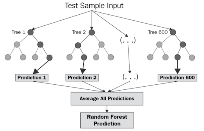
In the context of regression, Random Forest leverages the strength of multiple decision trees to make accurate and robust predictions by averaging the outputs of numerous trees.

This method is particularly effective in handling complex datasets with high dimensionality and non-linear relationships
Importance and applications
Random Forest Regression is important due to its ability to provide accurate and reliable predictions in various complex scenarios.
Its ensemble approach, which combines multiple decision trees, enhances the model's robustness and reduces the likelihood of overfitting. This makes it particularly valuable in handling datasets with high dimensionality and intricate, non-linear relationships.
Additionally, Random Forest Regression requires minimal data preprocessing, making it a practical choice for many real-world applications.
Theory Behind Random Forest Regression
Random forest regression is a supervised learning algorithm and bagging technique that uses an ensemble learning method for regression in machine learning. The trees in random forests run in parallel, meaning there is no interaction between these trees while building the trees.
Basics of Decision Trees
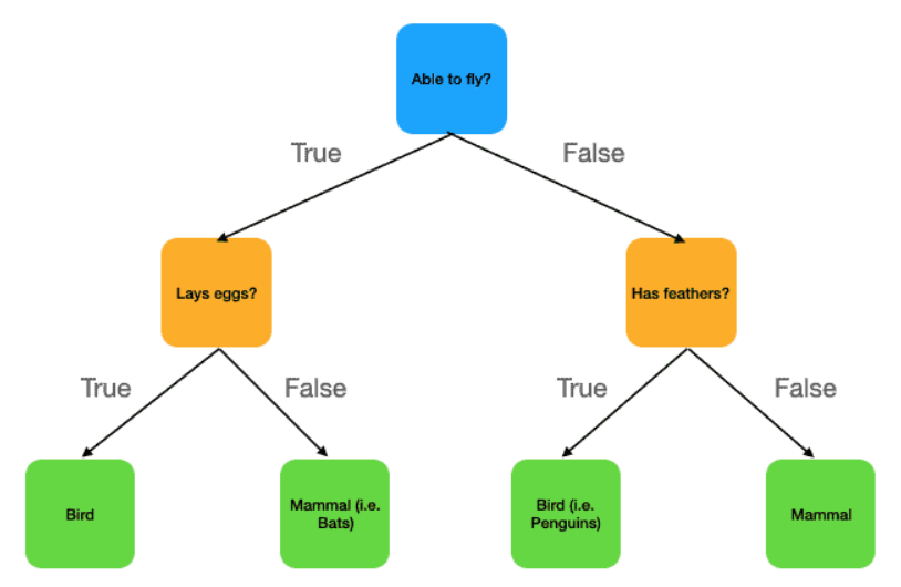
Decision trees are a type of algorithm used in machine learning for making decisions or predictions. They work by splitting data into branches based on certain conditions, much like a flowchart.
Root Node: This is the starting point of the tree, representing the entire dataset. It contains the first question or condition that splits the data.
Branches: These are the outcomes of the decision nodes, leading to further nodes or to a leaf. Each branch represents a possible decision or path.
Decision Nodes: These are the points where the data is split based on certain features or conditions. Each decision node represents a test on an attribute.
Leaf Nodes: These are the end points of the tree, where a final decision or prediction is made. In regression, the leaf node contains a numerical value, while in classification, it contains a category or class label.

Ensemble Learning
Ensemble Learning is a technique in machine learning where multiple models (often called "weak learners") are combined to solve a problem and improve the performance compared to a single model.
Types of Ensemble Learning -
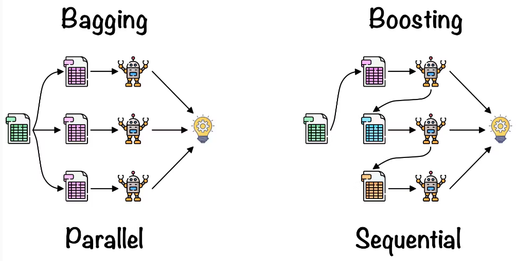
Bagging: This method involves training multiple models on different subsets of the data (created by random sampling) and then combining their results, usually by averaging or voting.
Random Forest Regression is based on Bagging.
Boosting: It trains models sequentially, with each new model focusing on correcting the errors made by the previous models.
Popular algorithms like AdaBoost and XGBoost are based on this method.

Bootstrapping
Bootstrapping is a statistical technique where multiple samples are created from an original dataset by randomly selecting data points with replacement. These bootstrapped samples are then used to train different models.
It helps to estimate how well a model performs by testing it on slightly varied versions of the data. By averaging the results of models trained on these samples, we get a more accurate and reliable estimate of the model’s performance.
Bootstrapping is often used in bagging to improve accuracy and reduce overfitting.
Implementing Random Forest Regression in Python
We are going to build a Random Forest Regression model to predict popularity of music. We are going to use a spotify dataset - Check here
Importing the dataset using pandas
import pandas as pd
spotify_data = pd.read_csv("/content/drive/My Drive/Spotify_data.csv")
Then, after we preprocess the data, we decide to take the following features -
Energy
Valence
Danceability
Loudness
Acousticness
Tempo
Speechiness
Liveness
Now we will build and train the Random Forest Regression model using sci-kit learn library.
Importing all the required packages from sci-kit learn:
from sklearn.model_selection import train_test_split
from sklearn.preprocessing import StandardScaler
from sklearn.ensemble import RandomForestRegressor
from sklearn.metrics import mean_squared_error, r2_score
from sklearn.model_selection import GridSearchCV
Fitting data to the model:
features = ['Energy', 'Valence', 'Danceability', 'Loudness', 'Acousticness', 'Tempo', 'Speechiness', 'Liveness']
X = spotify_data[features]
y = spotify_data['Popularity']

#dividing the dataset into training data and test data
X_train, X_test, y_train, y_test = train_test_split(X, y, test_size=0.2, random_state=42)

#scaling the datas to avoid biasing
scaler = StandardScaler()
X_train_scaled = scaler.fit_transform(X_train)
X_test_scaled = scaler.transform(X_test)
When training machine learning models, especially ones like Random Forest, the performance of the model is highly dependent on the values of its hyperparameters.
Instead of manually testing one value at a time, Grid Search will try all combinations of the provided values to find the best model configuration based on a performance metric.
param_grid = {
    'n_estimators': [50, 100, 200], # 3 values
    'max_features': ['auto', 'sqrt', 'log2'], # 3 values
    'max_depth': [10, 20, 30, None], # 4 values
    'min_samples_split': [2, 5, 10], # 3 values
    'min_samples_leaf': [1, 2, 4] # 3 values
}
The total number of combinations to be evaluated would be:
$$3\times3\times4\times3\times3 = 324$$
Grid Search will train the model 324 times (one for each combination of the parameters) and select the best set based on a chosen metric (like accuracy or mean squared error).
Training the model:
grid_search_rf = GridSearchCV(RandomForestRegressor(random_state=42), param_grid, refit=True, verbose=2, cv=5)
GridSearchCV: This is a tool in Scikit-learn that systematically works through multiple combinations of hyperparameters in a model, cross-validating each combination to find the one that performs best.
RandomForestRegressor(random_state=42): This initializes a Random Forest Regressor model.
param_grid: This is the dictionary of hyperparameters we are passing to the grid search, which defines the range of hyperparameters to be tested.
refit=True: This means once the grid search finds the best hyperparameters based on cross-validation, it will automatically refit the model using the entire training set and the best hyperparameters found.
verbose=2: This controls the verbosity of the output. (A higher verbosity value gives more details on the progress of the grid search)
cv=5: The dataset will be split into 5 parts, and the model will be trained 5 times, each time using 4 parts as training data and the remaining 1 part as validation data.
grid_search_rf.fit(X_train_scaled, y_train)
# This line fits the grid search model to the training data.

best_params_rf = grid_search_rf.best_params_
#This line retrieves the best hyperparameters found by the grid search.

best_rf_model = grid_search_rf.best_estimator_
# This line retrieves the best model found during the grid search process.

y_pred_rf = best_rf_model.predict(X_test_scaled)
# This line makes predictions using the best model found by the grid search.
Now the model is complete, let’s calculate the error and check our predictions through plots.
from sklearn.metrics import r2_score
r2 = r2_score(y_test, y_pred_rf)
print(f"R-squared: {r2}")

plt.figure(figsize=(8,4))
plt.scatter(y_test, y_pred_rf, alpha=0.7)
plt.plot([y_test.min(), y_test.max()], [y_test.min(), y_test.max()], color="red", lw=2)
plt.xlabel('Actual Popularity')
plt.ylabel('Predicted Popularity')
plt.title('Actual Popularity vs Predicted Popularity (Best Random Forest Model)')
plt.show()

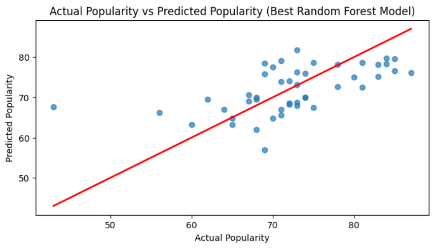
This plot shows how closely the predictions made by the best Random Forest Model (y_pred_f) match the actual values (y_test).
The red diagonal line represents perfect predictions.
Points closer to the red line are predictions that are close to the actual value, points farther from the line indicate larger prediction errors, and points on the line are accurate predictions.
Advantages of Random Forest Regression
Robust to Overfitting: Random Forest reduces overfitting by averaging the predictions of multiple decision trees, making it more generalizable and reliable compared to individual trees.
Minimal Data Preprocessing Required: Random Forest doesn't require extensive data preprocessing like scaling, normalization, or making the data linear. It can handle data in its raw form, including categorical variables (though one hot encoding may still be needed), making it easier to implement.
Works Well with Missing Data: Random Forest can handle missing data by estimating values from other trees in the forest, which helps maintain performance even with incomplete datasets.
Limitations of Random Forest Regression
Computationally Expensive: Training a Random Forest can be slow and resource-intensive, especially with a large number of trees and a large dataset, as it involves building multiple decision trees.
Less Interpretable: While Random Forest provides good predictions, it's harder to interpret compared to simpler models like linear regression. The complexity of multiple trees makes it difficult to understand the reasoning behind individual predictions.
Not Ideal for Extrapolation: Random Forest struggles with extrapolation (predicting beyond the range of training data). It performs well for interpolation within the training data but may fail to predict accurately for unseen data points outside that range.
Applications of Random Forest Regression
Medical Diagnosis: In healthcare, Random Forest can predict patient outcomes or the effectiveness of treatments based on factors like medical history, test results, and demographics.
Sales Forecasting: Businesses use Random Forest to forecast future sales by analyzing past sales data, market trends, and customer behaviors, aiding in decision-making for inventory and marketing strategies.
House Price Prediction: Random Forest can be used to predict real estate prices by analyzing various factors like location, size, number of rooms, and neighborhood amenities, making it valuable in real estate analytics.
Conclusion
In conclusion, Random Forest Regression is a reliable and widely used algorithm for predicting continuous values across various fields. Its ability to handle complex, non-linear relationships, minimal preprocessing needs, and resistance to overfitting make it a strong choice for many predictive tasks. However, it's computationally intensive and less interpretable than simpler models. Despite these limitations, its versatility and accuracy in applications such as price prediction, medical diagnosis, and sales forecasting make it a valuable tool for data scientists and analysts.
So, this was quite an overview about Random Forest Regression in machine learning. After reading this blog, you should have a basic understanding of how Random Forest Regression works and how to implement it in Python for various applications.
If you have any questions or need further clarification on any of the topics discussed, feel free to leave a comment below or reach out to me directly. Let's learn and grow together!
LinkedIn: https://www.linkedin.com/in/utkal-kumar-das-785074289
To further explore the world of machine learning, here are some recommended resources:
Subscribe to my newsletter
Read articles from Utkal Kumar Das directly inside your inbox. Subscribe to the newsletter, and don't miss out.
Written by

Utkal Kumar Das
Utkal Kumar Das
🤖 Machine Learning Enthusiast | 🌐 aspiring Web Developer 🔍 Currently Learning Machine Learning 🚀 Future plans? Eyes set on mastering Competitive Programming, bagging internships, winning competitions, and crafting meaningful projects.