Lovelace's Program: Part 11 - the Language of the Table
 Greg Alt
This is the eleventh part of a series of blog posts taking a deep look into Ada Lovelace's 1843 computer program, starting with Part 1: First Look at the First Program.
In an earlier post I talked about the programming language that was used by Ada Lovelace in her table in Note G. As her table was the first computer program, this language was the first programming language. This language was given no name, so I’ll just refer to it as the “language of the table,” or LOTT for short.
Babbage’s ”Series L” notes show that he had developed each part of the notation as an evolving language, but he never put it all together in one table. Lovelace put it all together in her Note G table. In the text of her notes, she also documented much of the language for the first time. Neither gave a full specification, though.
I’ll try to fill that gap a bit by summarizing the different parts of the language. I’ll then follow up with an example table that renders the Mandelbrot Set, using only features used by Lovelace in her table to compute the Bernoulli numbers.
Which Language of Which Table?
First, I want to be clear about exactly which language I’ll be talking about and which one I’ll use in my example. Charles Babbage constructed a language with different features, some of which were supported by his design of the Analytical Engine at the time, and some of which didn’t make it into the design until much later than Lovelace’s publication in 1843.
I will be looking specifically at only features used explicitly by Lovelace in her table, along with one feature discussed in Note G and required to make her program run but not explicitly used in the table itself.
For example, Babbage’s design of the Analytical Engine included operations to “step up” and “step down” a variable, shifting it by some number of digits one way or the other. These were not used explicitly or implicitly in Lovelace’s program, so I am excluding them from LOTT. Even though they would have come in handy for my Mandelbrot Set example, I instead used multiplication and division by powers of ten as a less efficient equivalent operation.
Another feature, Lovelace’s use of auto-increment indexing, was essential to make her program work, and was documented in the text of Note G. She didn’t, though, introduce a notation to support it explicitly. I will address this awkwardness by introducing a simple notation, adding a right arrow next to a variable to indicate auto-increment addressing should be used as Lovelace described:
1v21→
This LOTT is what I support in the transliteration tool I showed in an earlier post. It takes a table in .csv format and generates compileable C code.
In short, the language uses the features used in Lovelace’s Note G table, with the one extension of an explicit notation for auto-increment addressing. Any other feature of the Analytical Engine, regardless of which design plan, is excluded from the language.
Four Parts of The Table
There are four parts to Lovelace’s table, each with its own rules and purpose. I’ll talk about each in turn.
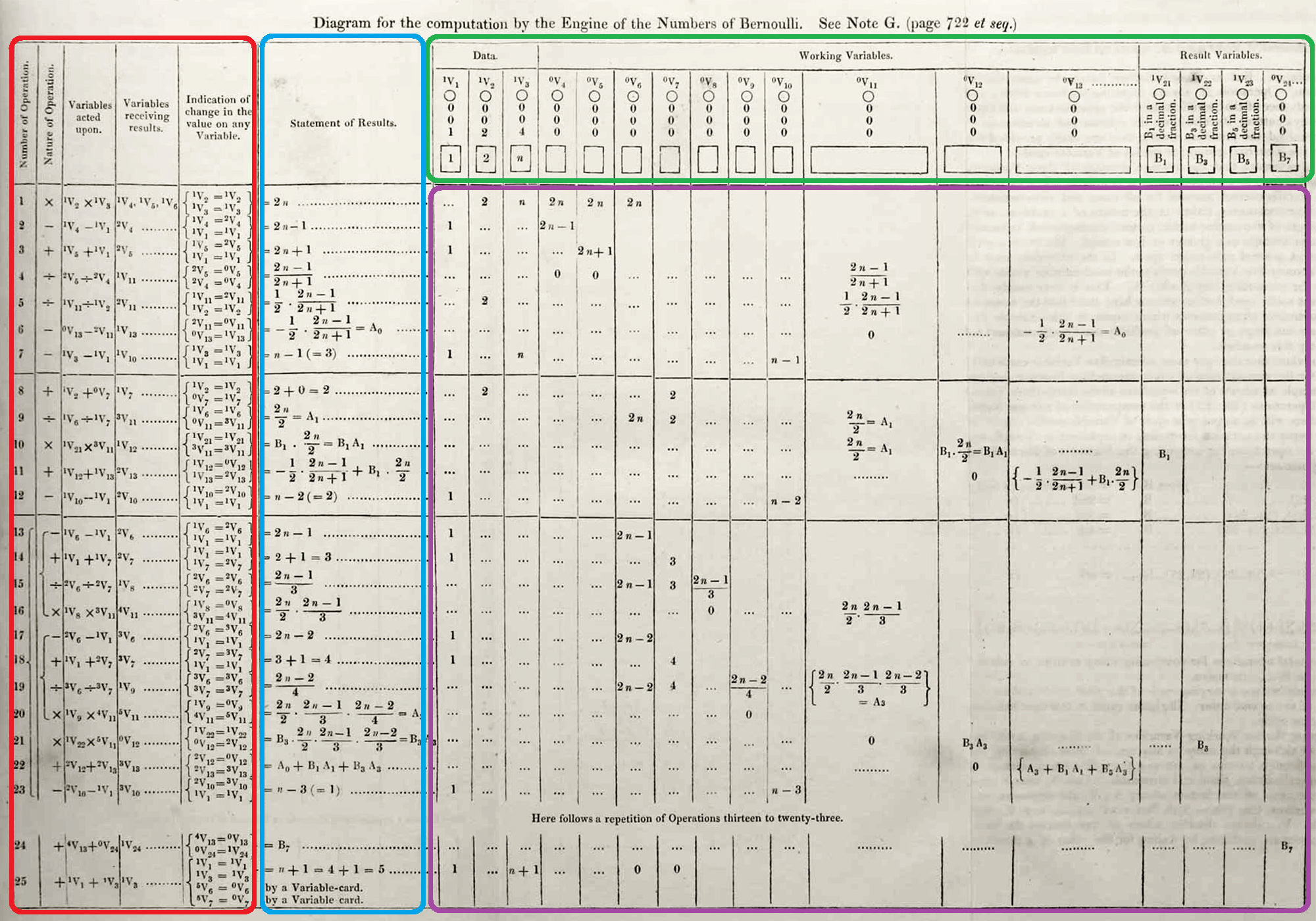
I’ll be using my own terminology for the different parts of the table, to be a bit more precise and explicit about the language structure than in Lovelace’s notes.
First, there’s the variable diagram in the upper right, marked off in green.
Next, there’s the table of operations, on the left side, in red.
Then there’s the Statement of Results column, in blue.
And finally, there’s the variable trace table, making up the bulk of the table, on the lower right, in purple.
Variable Diagram
Lovelace talks extensively about the diagram of variables in the upper right in her Note B and Note D.

The first thing to mention are the three classes of variables Lovelace describes in Note D:
Data: the input values to be set on the Analytical Engine before running
Working Variables: intermediate and temporary values used in the process of computing
Result Variables: the output generated by the program, to be read off at the end
You can think of these as variable declarations at the top of a function in a modern programming language. The Data must have values specified, while the rest are generally expected to be zero at the start. Lovelace clarifies in Note G that B1, B3, and B5 are given non-zero values under Result Variables to better show how the computation would look when calculating B7, but these are expected to be zero and filled in by the Analytical Engine.
Each variable declaration, then, is composed of four parts in a vertical column:
Variable: this consists of a left-superscript number that is either 0 or 1, followed by ‘v’ and then a lower subscript identifying the variable. If the variable starts with a value of 0, then the left-superscript should be 0. Otherwise, it should be 1 to indicate that the variable’s state has changed from an initial 0.
Sign: a circle that can have a + or - to indicate the sign of the value, or left blank to also mean positive. As Lovelace’s program did not use this, my python transliteration script assumes all Data variables start out with a positive value.
Digits: Lovelace’s table only includes three digits, for hundreds, tens, and ones place digits, so that’s what I support in my python script. Obviously, this could have supported any number of digits up to the full precision of the Analytical Engine.
Symbols: this square contains an arbitrary collection of symbols. They are not used in computation and are just a way to document the code for ease of reading. Lovelace uses this to mark constants like 1 and 2, but also variable names like n, B1, B3, etc.
It’s worth noting that only the Data variable declarations are used in computation, since they specify the initial values to be input.
Table of Operations

As I mention in my first post this part of the table is the core specification of the computations to be carried out.
There are five columns:
Number of Operation: like a simple modern line number, used to mark the start and end of a “Here follows…” loop.
Nature of Operation: the arithmetic operation to execute: +, -, *, /
Variables acted upon: this redundantly gives the operation, and also the two operand variables. The left-superscript is just to document the progression of the state of a variable. If it is 0, then the variable contains 0. Otherwise, the superscript increments each time the variable is assigned a new value. Only the right-subscript impacts computation itself as it specifies which variable is used.
Variables receiving results: one or more variable can receive the result of the operation. The left-superscript should be incremented one more than the previous occurrence of the same variable. If the variable receiving the results is not also one of the variables acted upon, then the variable is expected to have been set to zero before being assigned to. This is quirk of the Analytical Engine hardware that modern programmers wouldn’t be familiar with.
Indication of change in the value on any Variable: this column is described by Lovelace in Note D. It can be a bit confusing to modern programmers, but just remember that the Analytical Engine when operating on a value from a variable can cause that variable to retain it’s value or set it to zero, based on different variable cards. This column primarily specifies if a variable acted upon is retained (1v1 = 1v1) or reset to zero (2v5 = 0v5). Note that a variable that is not used in the acted upon column can be zeroed here as well. Lastly, if a variable used in the acted upon column is also listed in the Variables receiving results column, then this assignment can be noted here as well (1v4 = 2v4). Curly braces are used here just as a visual grouping aid to make it clear which row the listed variables are on.
As I mentioned above, I’ve slightly extended the notation to allow explicit use of Lovelace’s idea of automatically advancing which variable is read from or written to. This is something similar to modern auto-increment addressing, useful for processing arrays of data without having to unroll loops. For this, appending a right arrow, →, after a variable in either the variables acted upon or variables receiving results columns means that the index of such variable should be understood to be repeatedly advancing with each use, as Lovelace described in Note G:
Operation 21 always requires one of its factors from a new column, and Operation 24 always puts its result on a new column. But as these variations follow the same law at each repetition (Operation 21 always requiring its factor from a column one in advance of that which it used the previous time, and Operation 24 always putting its result on the column one in advance of that which received the previous result), they are easily provided for in arranging the recurring group (or cycle) of Variable-cards.
In addition to the columns described above, there are a few other notations used in Lovelace’s table:
Solid horizontal lines: these mark conditional forward jumps, as explained in the text of Note G. The variable receiving results in the previous operation is checked to see if it is zero. If so, execution jumps forward to the operation just after the next “Here follows…” loop specification.
“Here follows a repetition of Operations thirteen to twenty-three” this marks a loop conditional. The variable receiving results in the previous operation is checked to see if it is zero. If it is not zero, then execution jumps backwards to the first operation of the loop. The first and last operation numbers for the loop are specified in as English words, such as “thirteen”.
Curly braces: curly braces are used a a visual aid to group operations for loops, such as between 13 and 23 above. They are also used to visually group 13 to 16 and 17 to 20—it’s not clear the meaning, but it seems to suggest a possibly reuse of operation cards with different variable cards. In general, curly braces don’t impact computation, and are just documentation for a human reading the code.
Statement of Results
This next column, Statement of Results, isn’t used for computation, but serves the same purpose as modern end of line comments in source code:

Looking at Lovelace’s table, you can see that she primarily tries to document the general case in terms of n, but often refers to her specific example of a snapshot in time of the calculation of B7.
At the end, you can see simple English-language notes of “by a Variable card.” This is a case where a variable is being zeroed even though it wasn’t mentioned in the Variables acted upon column, so it would require additional variable cards.
Variable Trace Table
Finally, the bulk of the space of the table is used for a trace table of all the variables used.
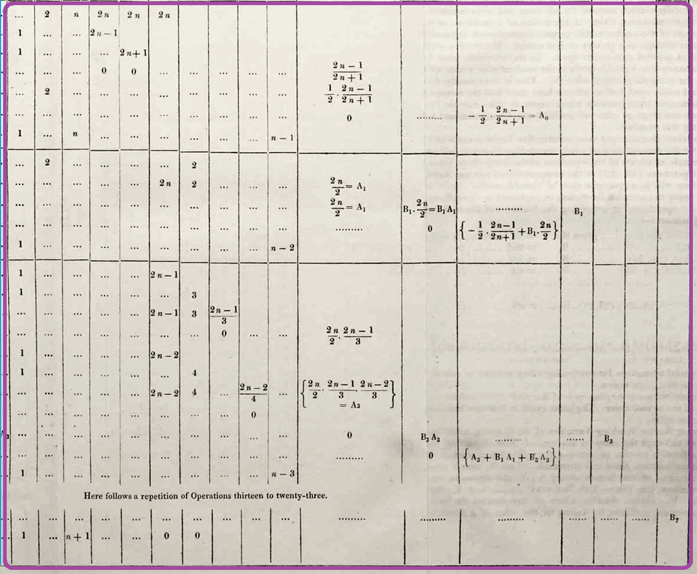
This trace table isn’t required for computation, but it’s useful to understand what’s expected to happen when reading the program. The value is updated in the appropriate row/column whenever a variable’s value changes in an operation. This can happen if it is assigned a value (mentioned in Variables receiving results column) or zeroed (mentioned in the Indication of change… column using a zero left-superscript on the right side of the equal sign).
Much like the Statement of results column, these values are usually given in general terms, such as in terms of n, rather than specific values. If a value doesn’t change in the given row, this can be indicated by leaving it blank, giving … or by restating the previous value.
Now that I’ve summarized the language of the table, I’ll give a new example table I made.
Computation by the Engine of the Set of Mandelbrot
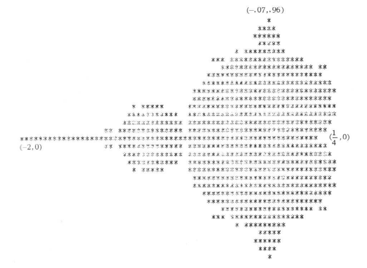
Just as Lovelace used an example from mathematics, calculating the Bernoulli numbers, I wanted to use another example from mathematics, this time more modern. While the “language of the table” that Lovelace used is Turing-complete, as I explained in a previous post, I wasn’t sure how easy it would be to construct a very different program using the same language. I chose something a bit more complex, calculating a 2D image of the Mandelbrot set, reproducing the results of the famous 1978 paper:
The Mandelbrot Set
You might have seen more colorful, high resolution images of some zoomed in parts of this fractal object, but I wanted something that was more feasible for the Analytical Engine’s display hardware.
You’ll remember that Babbage’s designs of the Analytical Engine called for as many as a thousand variables with each variable containing as many as 50 decimal digits. Each variable was implemented as a vertical stack of gears with its current digits visible through prisms. If you stood back, looking at the machine, this could be thought of as a display 50 “pixels” tall by 1000 wide, with each “pixel” being a digit between 0 and 9.
The image above of the Mandelbrot Set, as rendered by Robert Brooks and J. Peter Matelski for their paper, is 31 “pixels” tall by 68 wide. Each “pixel” is either a space or an asterisk, so two possible values. And the “display” was a printer.
If you are interested in learning more about the Mandelbrot Set, I suggest starting with the wikipedia page. For now, just know that a program to calculate such an image consists of two nested loops, looping over columns and rows. For each pixel, another loop is run that does some fancy math. A simple formula is followed using a complex number unique to each pixel:
z(n+1) = z(n)² + c
Both z and c are complex numbers, meaning they have two components, usually labeled a and b, in the form: a+bi
For each pixel, z starts at 0 and c is calculated where a corresponds to the pixel’s x coordinate and b corresponds to the pixel’s y coordinate. The above calculation is repeated and two possible things happen. For many initial values, z eventually grows large and just keeps growing bigger and bigger indefinitely. For other values, it bounces around and stays small forever. For some, it’s hard to know what it’s going to do because it takes a long time before it eventually gets large and then rapidly explodes from there.
The Mandelbrot Set is the set of complex numbers (pixels) that never get big. In practice we can’t be sure that they’ll never get big, but we can set some maximum number of iterations where we call it good enough. If the innermost loop runs that many iterations without blowing up, we’ll say that pixel is in the Mandelbrot Set. If the innermost loop blows up earlier, then we’ll say the pixel is not in the Mandelbrot Set. A simple measure of it’s blowing up or not is if the magnitude of z ever gets to be 4 or larger, then you know it will blow up.
In the 1978 paper, they assigned an asterisk for pixels in the Mandelbrot Set and a space for pixels not in it. One of the 1978 authors, in a recent StackExchange post, gave the specific parameters used, so I was able to use that as a starting point:
I can confirm that the programming constants used were indeed Δx=.035, Δy=1.66∗Δx. The grid center is (−.75,0) which is a boundary point by the way: it is exactly represented in floating point. The original iteration cap was 250.
The run date was 8 Jan 1979. It was my first computer M image using the now standard program. There has been lots of criticism of it, but it is clearly fine.
The font Lucida-console regular has aspect ratio very close to 1.66 Take Notepad or WinVi with this font and you have an effective previewer and printer in imitation of the lineprinter at Stony Brook in 1978.
Note: the UNIVAC mainframe had 36 bit single and 72 bit double precision. Of course, I ran both varieties. The modern choices are 32, 64, or 80 bit. Using 32 bit is problematic. --JPM
Compute the Mandelbrot Set in Modern C
Here’s an example of how you might compute the Mandelbrot Set in modern C:
#include <stdio.h>
int main(int argc, char **argv) {
    double center_ca = -0.75;
    double center_cb = 0.0;
    int xsteps = 68;
    int ysteps = 31;
    int maxiter = 250;
    double dx = 0.035;
    double aspect = 1.66;
    double dy = dx * aspect;
    double ca_start = center_ca - (xsteps*0.5+1.0)*dx;
    double cb_start = center_cb - (ysteps-1.0)*0.5*dy;

    char str[100] = {0};
    for(int x=0; x<xsteps; x++) {
        double ca = (double)x*dx+ca_start;
        for(int y=0; y < ysteps; y++) {
            double cb = (double)y*dy+cb_start;
            double za = 0.0f;
            double zb = 0.0f;
            int iter = 0;
            for(; iter < maxiter && za*za+zb*zb < 4.0; iter++) {
                double temp = za*za-zb*zb + ca;
                zb = 2.0*zb*za + cb;
                za = temp;
            }
            str[y] = iter < maxiter ? '0' : '1';
        }
        printf("%s\n", str); // print by column, so need to transpose text
    }
}
My Table for Computing the Mandelbrot Set
The C code above is a good starting point to figure out how to write it in the language of the table. So I knew I had to have three nested loops. Somehow I had to set individual digits in a series of variables. My strategy started from the idea that the outer loop would cycle over 68 different variables, using Lovelace’s auto-increment indexing idea. Each variable would be one column of pixels from the Mandelbrot Set, with 1 for pixels in the set and 0 for pixels outside.
Lovelace’s table had a loop that generated a series of values in successive variables, so I could do things much like she did.
The next loop would loop over 31 pixels within each column. I just used two nested “Here follows…” loops using variables acting as x and y counters, counting down to zero, because that’s what “Here follows…” expects.
For each pixel, I needed another loop. This would do some math in each iteration—that’s the easy part as it’s just a series of arithmetic operations on a few variables. And I could test against the maximum iteration count by counting down to zero as in the other loops—so a third “Here follows…” loop.
But how to break out early? For this I used a horizontal line which causes a forward jump to just after the loop if the previous operation’s result is exactly zero. That condition was a bit tricky to figure out. How do I do simple arithmetic on some arbitrary number and get exactly zero if and only if the value was greater or equal to four? So 3.9999 needs to give me something nonzero, but 4.0, 4.0003 and 28.9 all need to give exactly 0.0.
The answer is to use one of the quirks of fixed point math in our favor. Most modern computers use floating point which lets you get accurate numbers with a wide range of scales. Fixed point, on the other hand, has a fixed scale. Below that scale, you get what’s called underflow, where your variable becomes exactly zero.
Let’s say p is our value to test. If I take 1/p, I get a value that gets closer and closer to zero the bigger p is. If I divide by some large power of 10, I can shift that result. Values of p that are big enough will get underflow, so become exactly zero. Smaller values of p won’t result in underflow, so there will be a nonzero value. That plus avoiding division by zero is all I need to make my conditional jump exiting the inner-most loop before hitting the maximum number of iterations.
A similar trick can be used to look at the number of iterations and get either exactly 0 or exactly 1. This value of 1 or 0 can then be shifted to the right pixel location in a column by multiplying by powers of 10 again and adding in.
Since I needed 31 pixels, I used a fixed point precision of 50 total digits and 31 fractional digits. This gave me enough precision to do all of the math and resulted in the 31 digits to the right of the decimal point being my “pixels.”
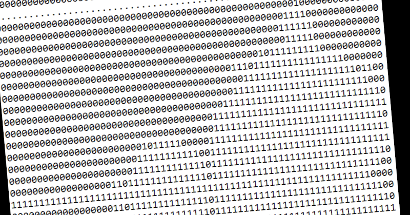
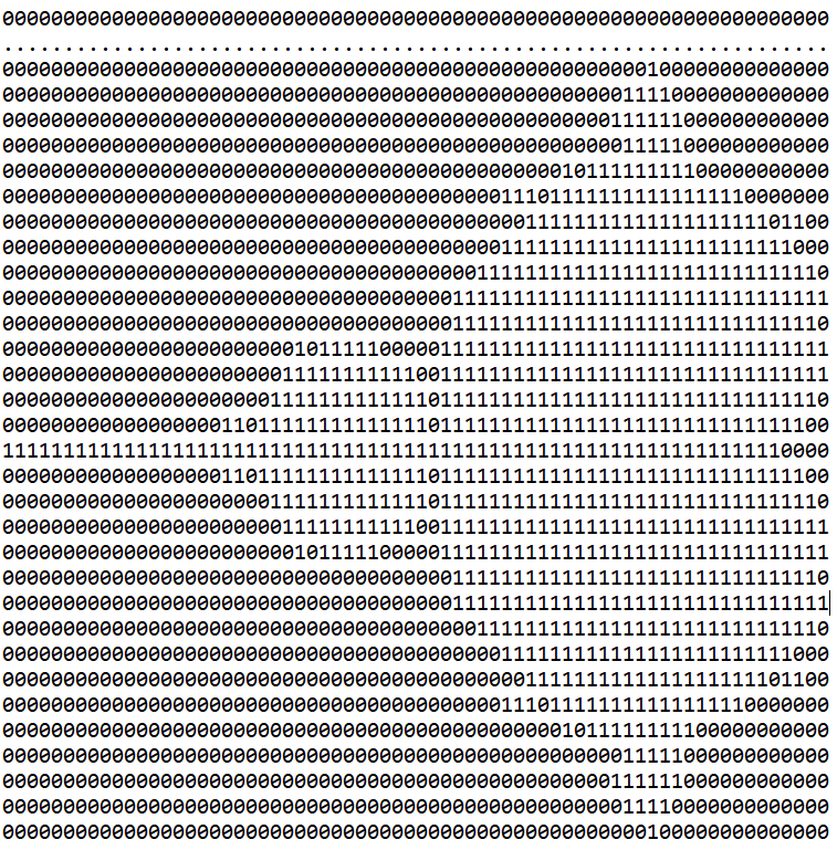
The result didn’t look quite right, though, when displayed the results:
0.0000000000000001000000000000000
0.0000000000000001000000000000000
0.0000000000000001000000000000000
0.0000000000000001000000000000000
0.0000000000000001000000000000000
0.0000000000000001000000000000000
0.0000000000000001000000000000000
0.0000000000000001000000000000000
0.0000000000000001000000000000000
0.0000000000000001000000000000000
0.0000000000000001000000000000000
0.0000000000000001000000000000000
0.0000000000000001000000000000000
0.0000000000000001000000000000000
0.0000000000000001000000000000000
0.0000000000000001000000000000000
0.0000000000000001000000000000000
0.0000000000000001000000000000000
0.0000000000000011100000000000000
0.0000000000000011100000000000000
0.0000000000000001000000000000000
0.0000000000000011100000000000000
0.0000000000000111110000000000000
0.0000000000001111111000000000000
0.0000000000011111111100000000000
0.0000000000001111111000000000000
0.0000000000011111111100000000000
0.0000000000011111111100000000000
0.0000000000011111111100000000000
0.0000000000011111111100000000000
0.0000000000011111111100000000000
0.0000000000001111111000000000000
0.0000000000001111111000000000000
0.0000000000001111111000000000000
0.0000000000000111110000000000000
0.0000000000000001000000000000000
0.0000000000011111111100000000000
0.0000000001111111111111000000000
0.0000000001111111111111000000000
0.0000000011111111111111100000000
0.0000000011111111111111100000000
0.0000010111111111111111110100000
0.0000010111111111111111110100000
0.0000011111111111111111111100000
0.0000001111111111111111111000000
0.0000011111111111111111111100000
0.0000111111111111111111111110000
0.0000011111111111111111111100000
0.0000111111111111111111111110000
0.0000111111111111111111111110000
0.0010111111111111111111111110100
0.0111111111111111111111111111110
0.0111111111111111111111111111110
0.1111111111111111111111111111111
0.0111111111111111111111111111110
0.0011111111111111111111111111100
0.0000111111111111111111111110000
0.0000011111111111111111111100000
0.0000011111111111111111111100000
0.0000011111111111111111111100000
0.0000011111111111111111111100000
0.0000001111111111111111111000000
0.0000001111111111111111111000000
0.0000000111111111111111110000000
0.0000001111111110111111111000000
0.0000001011111110111111101000000
0.0000000011111100011111100000000
0.0000000001011000001101000000000
There are a couple reasons for that. When I printf a variable in C++, it is displayed horizontally, but the Analytical Engine displays it’s variables vertically. So I have to transpose the output, turning rows into columns.
The other issue is the original paper knew their printer didn’t have perfectly square characters in its font. They had determined that each character was 1.66x as tall as it was wide and baked that aspect ratio into their calculations. I used the same ratio for my calculation. The result above gets the aspect ratio backwards and doubles up the error.
Transposing the result gets me something much better, especially when rendered in notepad:
The Table
Here’s my Mandelbrot Set table program as a spreadsheet.
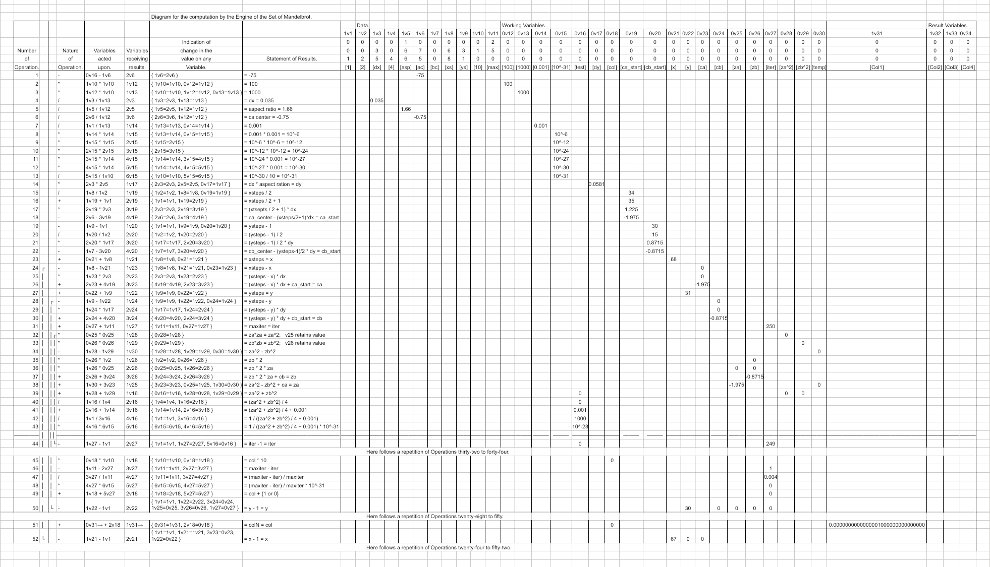
To run it, you need to export to .csv, run through my transliteration python script, and finally modify the resulting C code to use a C++ FixedPoint class with 50 digits of precision, 31 fractional, printing the result variables.
If someone ran this on a real Analytical Engine, there would be no need to print anything as the variables would be physically visible.
See my previous posts for how to add FixedPoint and for the python transliteration script.
Notably, I was able to run my new table with an unmodified version of the transliteration script, proving that the virtual machine Lovelace was programming for was enough to generate the Mandelbrot Set, even if the math would take another hundred years or so to be understood.
How long would this have taken on a real Analytical Engine? Well, let’s be lucky we live in an age of fast computers. Here are the statistics:
Multiplications: 1,033,392
Divisions: 412,911
Additions: 828,122
Subtractions: 415,918
At 1 minute per multiplication and division, that's over 2.7 years. But much faster than calculating it by hand, I’m sure.
Programming in the Language of the Table is Hard
Writing this table program gave me a new respect for Ada Lovelace. Even cheating by running it to test, it still took considerable effort to get right. And I’m sure there are still bugs, and certainly less than ideal code. I also took advantage of spreadsheet software to insert rows and do search and replace rather than tediously recopying and correcting errors with pencil and eraser.
Even with these extra tools at hand, I still found myself in dismay at having got into amazing quagmires and botheration. The satisfaction, though, of seeing the final output, 2.7 compute-years later, was worth it.
It’s been a long road digging into Ada Lovelace’s 1843 program to get a thorough understanding. I think it’s a good time to take a step back and, in my next post, look at her work in context with the first programmers of the 20th century.
Subscribe to my newsletter
Read articles from Greg Alt directly inside your inbox. Subscribe to the newsletter, and don't miss out.
Written by
