Welcome to Part 2.2 of Machine Learning!

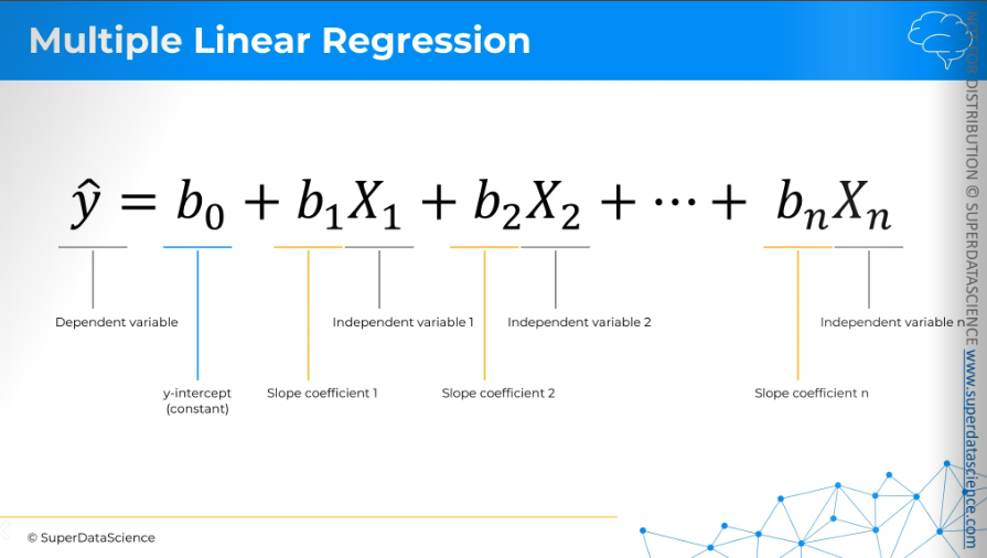
Here is the equation for multiple linear regression. As you can see, it is quite similar to our linear regression model.

Assumptions of linear regression

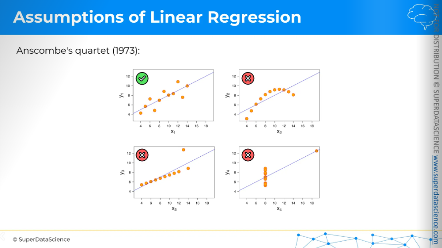
Now, let's look at the first dataset for the linear regression model assumption.

The first dataset is working well and serving its purpose. But look at the other datasets. They are not serving their purpose and are misleading. So, we shouldn't use linear regression in those cases.

These four datasets are known as Anscombe's quartet, and they show that you can't just blindly use linear regression everywhere. You need to make sure your dataset is suitable for linear regression. That's why the assumptions of linear regression are important.

Now let’s learn about them

Linearity

(Linear relationship between Y and each X)

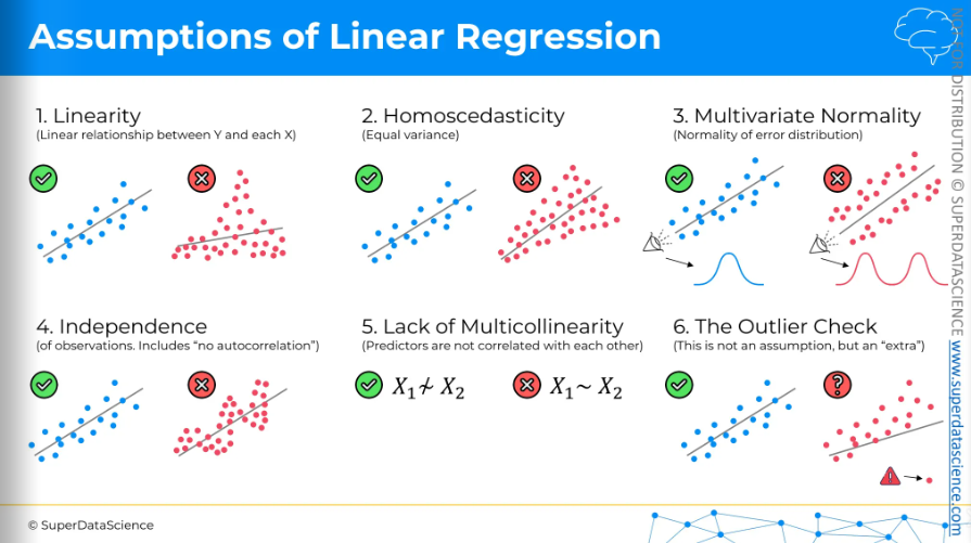
The first assumption is linearity. We need a linear relationship between the dependent and each independent variable.
Homoscedasticity

(equal variance)

Even though it sounds complex, homoscedasticity simply means equal variance. You don't want to see a cone shape on your chart, whether increasing or decreasing, as it means variance depends on the independent variable. In this case, we wouldn't use linear regression.
Multivariate Normality

(Normality of error distribution)

If you look at the chart on the right, something seems off. Ideally, along the line of linear regression, you should see a normal distribution of data points. Here, it's different, so we wouldn't use linear regression.
Independence

(of observation. Includes “no autocorrelation”)

We don't want any pattern in our data. A pattern indicate that rows are not independent, meaning some rows affect others. A classic example is the stock market, where past prices influence future prices. In such cases, we wouldn't use a linear regression model.
Lack of Multicollinearity

(predictors are not correlated with each other)

The fifth assumption is lack of multicollinearity. We want our independent variables or predictors not to be correlated. If they're not correlated, we can build a linear regression. If they are, the coefficient estimates in the model will be unreliable.
The outlier Check

(this is not an assumption, but an ‘extra’)

The sixth point is checking for outliers. This isn't a real assumption but an extra step to remember when making linear regression models. If you look at the chart, you can see the outlier is greatly affecting the regression line. So, we need to decide whether to remove outliers before making the model or keep them in. This choice depends on your understanding of the business and the data set.

Multiple Linear Regression Intuition

Dummy Variables

We gonna learn about dummy variables here. Here we have information on each company's profit, along with their spending on R&D, administration, and marketing. These are the expenses the company has, and then there's the state where it operates, either NY or California. Our challenge is to see if there's any connection between profit and all these variables, and if we can create a model to predict profit. So, profit is our dependent variable, and the blue ones are independent variables. We need to build a linear regression model.

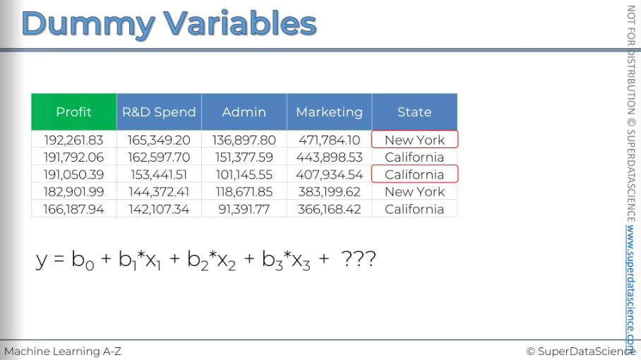
Now, for the equation: Y is our profit. Then, we have the B1 coefficient times the X1 variable, which is the R&D spend. X1 represents the dollar amounts in the R&D column. Then, there's the Admin variable, which is X2, so that’s how the equation is. But for the state, we have to figure out what we should place here.

So the approach you need while facing categorical variable is to create a dummy variable. First, identify each categorical value and create a column for each one. Here, we have only New York and California, so we build columns for them (we are kind of expanding our dataset)

Now to fill up the column (this is very interesting actually) - Put a 1 in the New York column for New York and 0 for everything else. Do the same for California

Now these two columns are called dummy variables. Building your regression model from here is very simple. All you need to do is use the New York column instead of the state names. You add a variable that is multiplied by D1, which is your dummy variable for New York. You don't use the California column either.

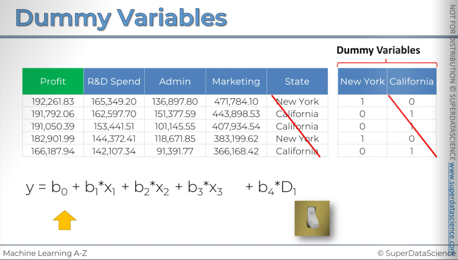
So, as you can see, all the information in our data is kept intact. If we just stick to the one New York column, you can tell right away if D1 is 1 then it's a company that operates in New York. If D2 is a 0 it's a company that operates in California.

We didn't lose any information by only including the New York column.

[Trick: Another thing I want to say is that dummy variables work like a switch. If the value is 1, the switch is on, meaning the company operates in New York. If the value is 0, it means the switch is off, indicating the company does not operate in New York]

Dummy Variable Trap

Do not use multiple dummy variables. You can never include both the dummy variables at one. In our example, we used NY only and found b4D1.

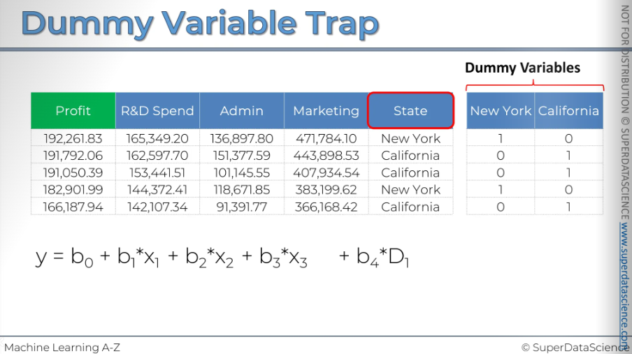
When one or more independent variables in a linear regression predict another, it's called multicollinearity. Because of this, the model can't tell the difference between the effects of D1 and D2. As a result, it won't work properly. This is known as the dummy variable trap.

[If you do the math, you'll see the real issue: you can't have the constant and both dummy variables in your model simultaneously]

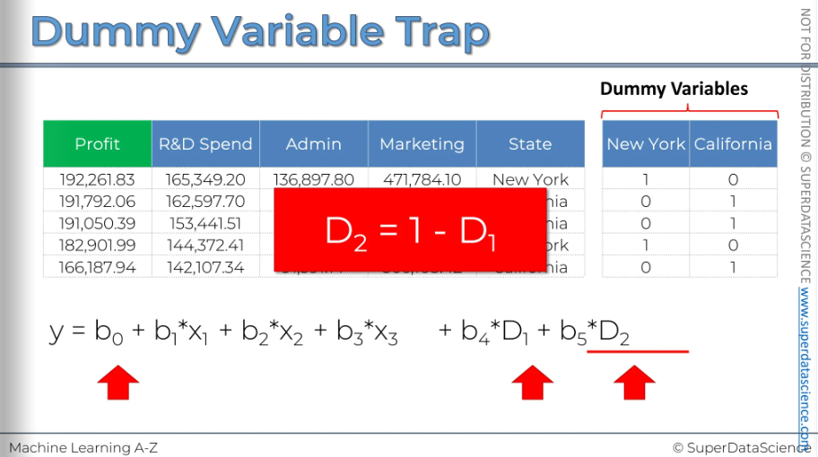
To sum up, when building a model, always include only one less than the total number of dummy variables in a set. If you have nine, include eight; if you have 100, include 99. Apply this rule to each set of dummy variables.

I hope this explanation was helpful and that you will never fall victim to the dummy variable trap in your modeling.

P - value

A P-value is a statistical measure that helps you understand the significance of your research results. It shows the chance of seeing the data, or something more extreme, if the null hypothesis is true. Simply put, a low P-value (usually ≤ 0.05) means there is strong evidence against the null hypothesis, suggesting you might want to reject it. On the other hand, a high P-value means the data fits well with the null hypothesis, indicating there's not enough evidence to reject it.

P-values are often used in hypothesis testing to help researchers make conclusions from their data.

Model Building

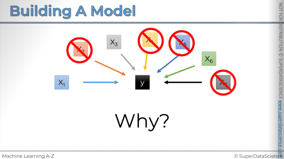
Do you remember the good old days when we had just one dependent variable and one independent variable? Everything was simple, and we only had to build a straightforward linear regression. It worked perfectly.

But now, our data has many columns. Those easy days are over, and all these columns could be predictors for a dependent variable. There are so many of them, and we need to decide which ones to keep and which ones to discard.

You might wonder why we need to remove columns or get rid of data. Why can't we just use everything in our model?

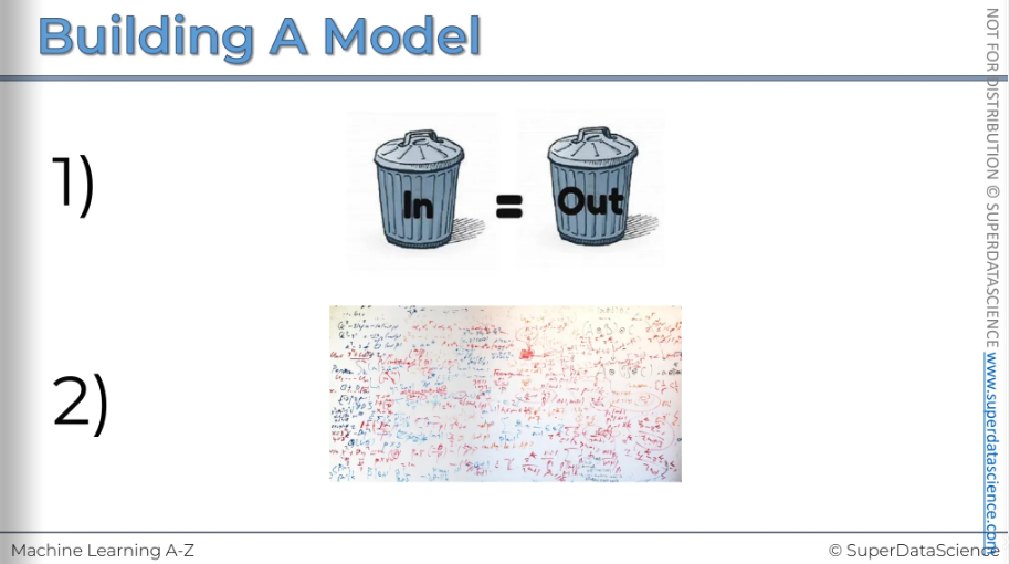
Well, I can think of two reasons right away.

First, "garbage in, garbage out." If you add too much unnecessary data, your model won't be reliable; it'll be a "garbage model."

Second, at the end of the day, you'll need to explain these variables and understand what they mean in predicting your dependent variable's behavior. Explaining a thousand variables isn't practical, so keep only the important ones that actually predict something.

There are five rules to build a model.

[Sometimes you'll hear about stepwise regression, which actually refers to steps 2, 3, and 4, as it follows true step-by-step methods]

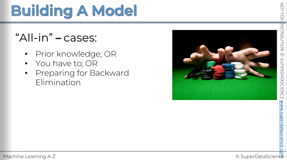
Method number one: All In.

This isn't a technical term; I just call it "all in." Basically, it means throwing in all your variables. This is something we just discussed that we shouldn't do.

When would you use this method?

One reason is if you have prior knowledge. If you know these variables are true predictors, you don't need to build anything new. You might know this from domain knowledge, past experience, or because someone provided these variables for the model. In that case, you just build the model.
Another reason could be if your company has a framework requiring these variables. It's like prior knowledge, but not your choice. For instance, a bank might need to use specific variables to predict loan defaults.
Lastly, you would use this method if you're preparing for a backward elimination type of regression, which is our next topic.

So, let's move on to backward elimination.

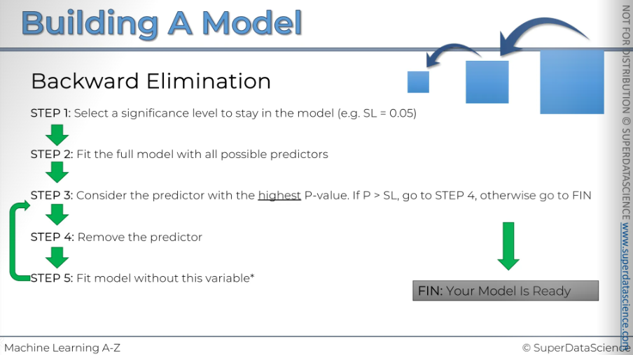
After Step 5, you go back to Step 3.

Once again, look for the variable with the highest p-value in your new model. Remove it. This is essentially Step 4, where you take out the variable.

Then, fit the model again with one less variable. Keep repeating this process until you reach a point where even the variable with the highest p-value is still less than your significance level.

If the condition where p is greater than the significance level is not met, then you don't proceed with Step 4 anymore. You move to the end, and in this case, "end" means finish.

Your model is ready when all the remaining variables have p-values less than the significance level.

That's how the backward elimination method works. Let's move on to the next one.

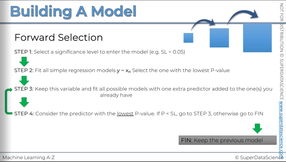
We started with Step 1:

Select the significance level to enter the model. In this case, we choose 5 percent.

Next, we move to Step 2:

We fit all possible simple regression models. This means we take the dependent variable and create a regression model with each independent variable we have. From all these models, we select the one with the lowest p-value for the independent variable. As you can see, this involves a lot of work.

Then, we proceed to Step 3:

We keep the variable we've just chosen and fit all other possible models by adding one extra predictor to the one we already have.

What does this mean?

It means we've selected a simple linear regression with one variable. Now, we need to construct all possible linear regressions with two variables, where one of those variables is the one we've already selected. Essentially, we add each of the other variables one by one. We decide, "Let's add this variable," and then, "Let's add the next one," but separately. We construct all possible two-variable linear regressions while definitely keeping the variable we've already selected.

So, what do we do after that?

Out of all these possible two-variable regressions, we consider the one where the new variable we added has the lowest p-value. If that p-value is less than our significance level, it means the variable is significant, so we go back to Step 3.

What does that mean?

It means we now have a regression with two variables, and we will add a third variable. We'll try all possible remaining variables as our third variable. From all these models with three variables, we'll proceed to Step 4 and select the one with the lowest p-value for the third variable we added.

We continue this process. Essentially, we keep expanding the regression model by carefully selecting from all possible combinations, adding one variable at a time. We stop when the variable we add has a p-value greater than our significance level. When this condition is not met, we don't return to Step 3; we finish the regression. Why? Because the variable we just added is no longer significant. We also know we selected the one with the lowest p-value, so there is no other variable we can add that will have a p-value less than our significance level in any further regression.

From this point on, the new variable will always be insignificant.

So, this is where we finish the regression.

The key is to keep the previous model, not the current one.

This makes sense because you've just added an insignificant variable. So, there's no point in keeping it; just go back one step.

That's how forward selection works.

I know it can be a bit confusing, but try to understand and maybe read these instructions again.

It makes more sense when you picture what is happening.

And next we're moving on to the bidirectional limit elimination.

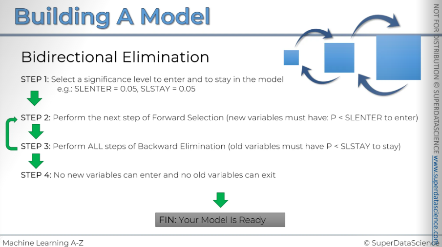
This method combines two steps. First, choose a significance level for entering and staying in the model. Use the same level for both. New variables must have a significance level lower than the entry threshold to be added.

Next, perform backward elimination. Try to remove unnecessary variables, then return to add another variable. Each time you add a variable, perform backward elimination again. Remove variables if possible, then return to add more.

Continue this iterative process until you can't add or remove variables. At this point, your model is complete. This method can be tedious, so it's best handled by a computer. This is how bidirectional elimination, or stepwise regression works.

And finally, let's discuss all possible models.

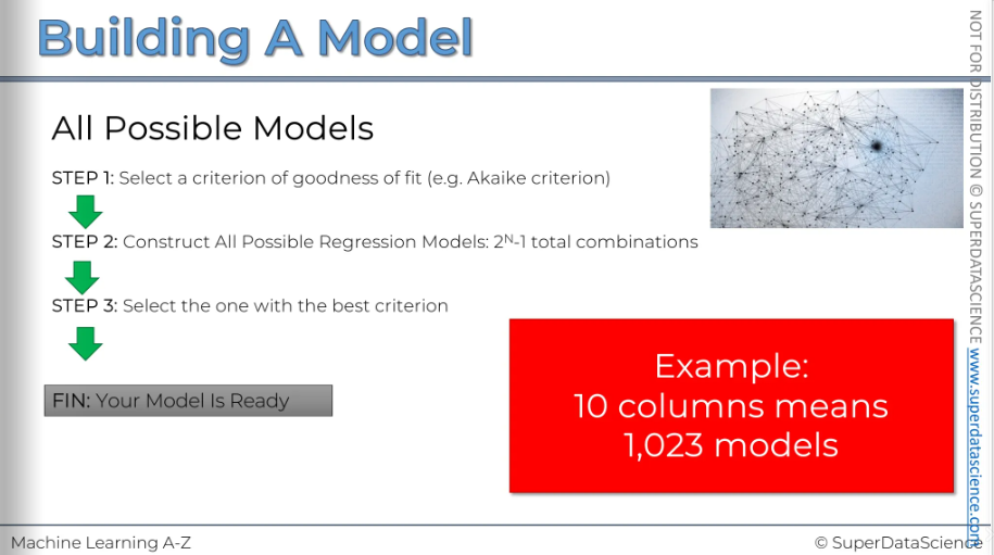
This is probably the most thorough approach, but it's also the most resource-intensive. You start by selecting a criterion for goodness of fit, like the R-squared value. There are many different criteria you can choose from. Then, you construct all possible regression models. If you have 'n' variables, there will be 2 to the power of 'n' minus one total combinations of these variables. That's exactly how many models there can be. In the final step, you select the model with the best criterion.

There you go, your model is ready.

It sounds easy, but let's look at an example. Even if you have 10 columns in your data, you'll have 1,023 models. That's an enormous number of models. And we're not even talking about columns you've already filtered out. For instance, in our example, you might have five or six columns. Now, imagine when you get a dataset that you need to analyze, which typically has around 100 columns. That is INSANE!

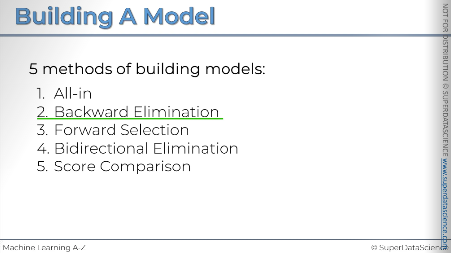
In conclusion, we have five methods for building models: backward elimination, selection by direction, and score comparison.

Multiple Linear Regression in Python

Resources :

Google Colab file: https://colab.research.google.com/drive/1Lp16gstLKT6DfhTPNsbwdG3BgEjWDZIO (copy this file)
Datasheet: https://drive.google.com/file/d/1-RL-SsWNo0PhP_goWfXrwnauRuFDidl9/view (download and upload in colab file)
Data preprocessing template: https://colab.research.google.com/drive/17Rhvn-G597KS3p-Iztorermis__Mibcz

In this dataset, each row represents a startup. For each startup, data scientists collected information on R&D spending, administration spending, marketing spending, the state, and profit. The goal is for the VC fund to decide which startup to invest in based on this information. We have data from 50 startups. If you train a model to understand these correlations, you can use it to predict the profit of a new startup. And yes, after copying the colab file, delete all the code cells. Just the code cells, not the text cell.

Code implementation:

First of all, we need to copy paste our templates into our colab file.

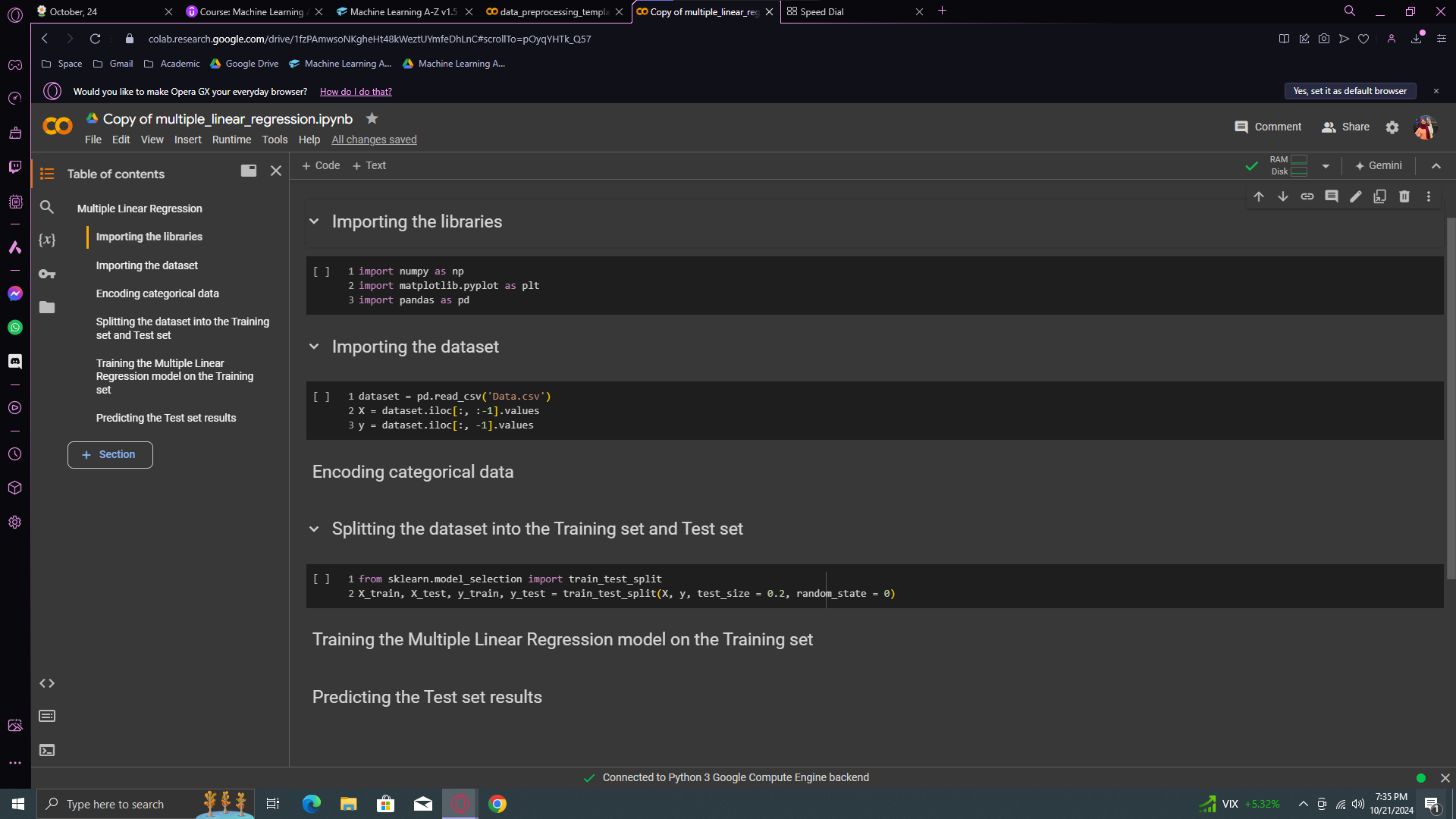
Now, change the datasheet name to 50_Startsup. Okay, then move to the encoding categorical part and copy paste the OneHotEncoder from your data preprocessing file (we did it on the first blog)

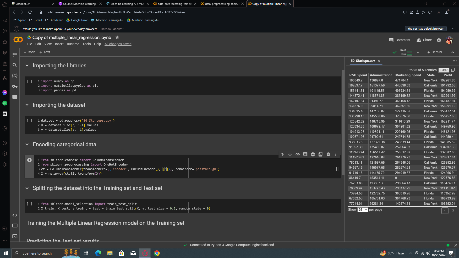
Here, we just have to change the column which we want to one hot encode. According to the previous one, the data had categorical values on the index of 0. In our current sheet, the categorical value is on the 3rd column.

Now let’s print X. Run all the cells and you will see your categorical data has been transformed beautifully.

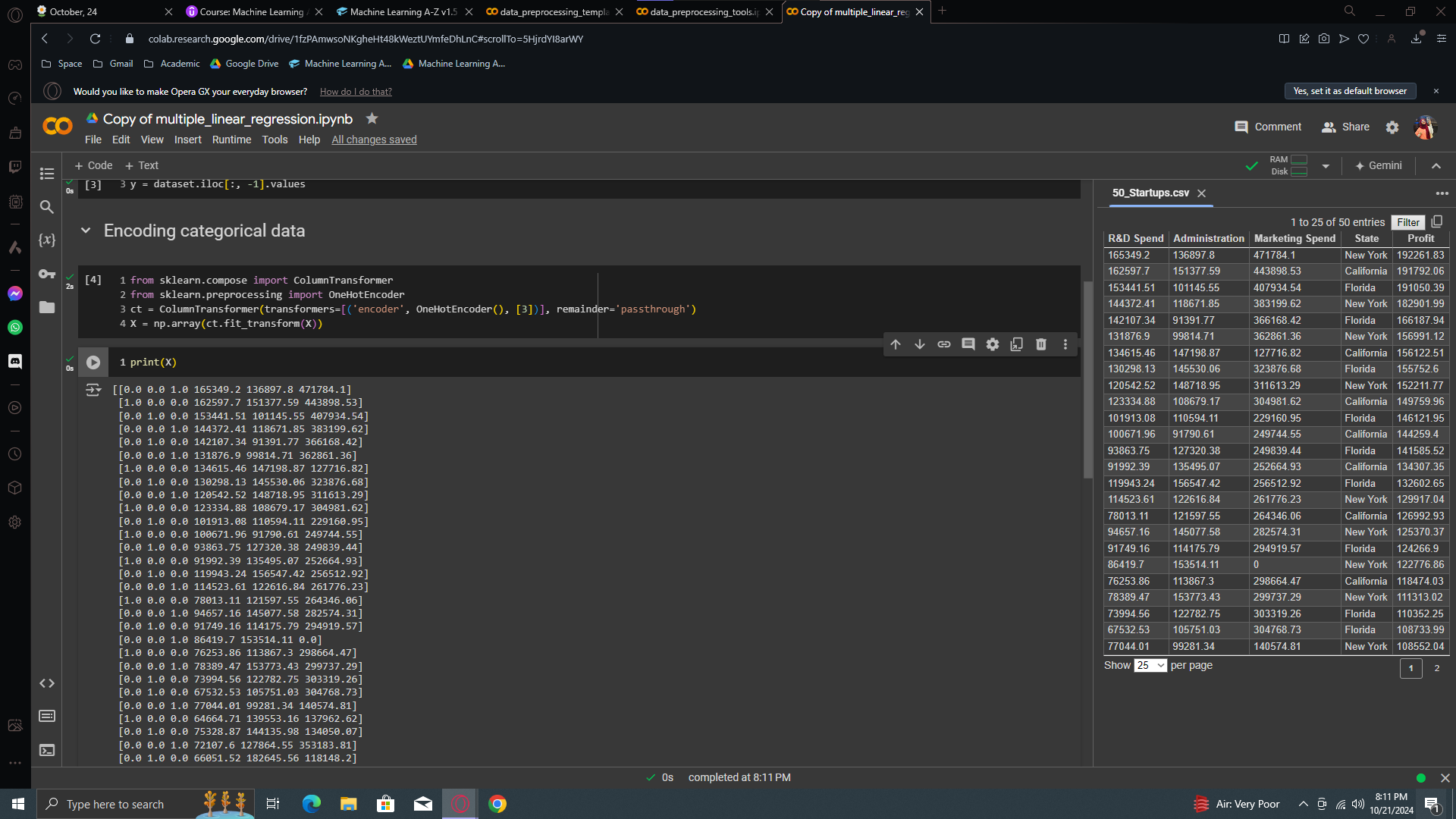
Looking at our dataset, the first row has "New York" as a state, encoded as 0, 0, 1. The second row has "California," encoded as 1, 0, 0. Lastly, "Florida" is encoded as 0, 1, 0. That's the one-hot encoding, and now we have a fully pre-processed dataset.

IMPORTANT

We don't need to apply feature scaling. In Multiple Linear Regression, coefficients adjust for different feature values, so scaling isn't necessary.
Do we need to check the assumptions of linear regression? The answer is absolutely not.

(Don't worry about Multiple Linear Regression assumptions. If your dataset has linear relationships, the regression will work well and be accurate. If not, it will perform poorly, and you can try another model. That's it.)
Do we have to do anything to avoid the dummy variable trap? The answer is no.

The class we have important to work with multiple linear regression is trained on several actions. So don’t worry about it. The redundant one will be outcaste automatically.
Do we have to work on selecting the best feature?

Why? For the exact same reason as the dummy variable trap. Our class will automatically detect the best feature, you know, the feature with highest P - value/ the most statistically significant to figure out how to predict the dependent variable and so on.

Okay, now let’s move to building model. But before that, I have a good news. The class we're about to use for building and training this Multiple Linear Regression model is the same as for the Simple Linear Regression model. It will recognize multiple features for multiple linear regression, but everything else remains the same. All your features and the profit, your dependent variable, will be handled. It will manage the dummy variable trap and select the most statistically significant features.

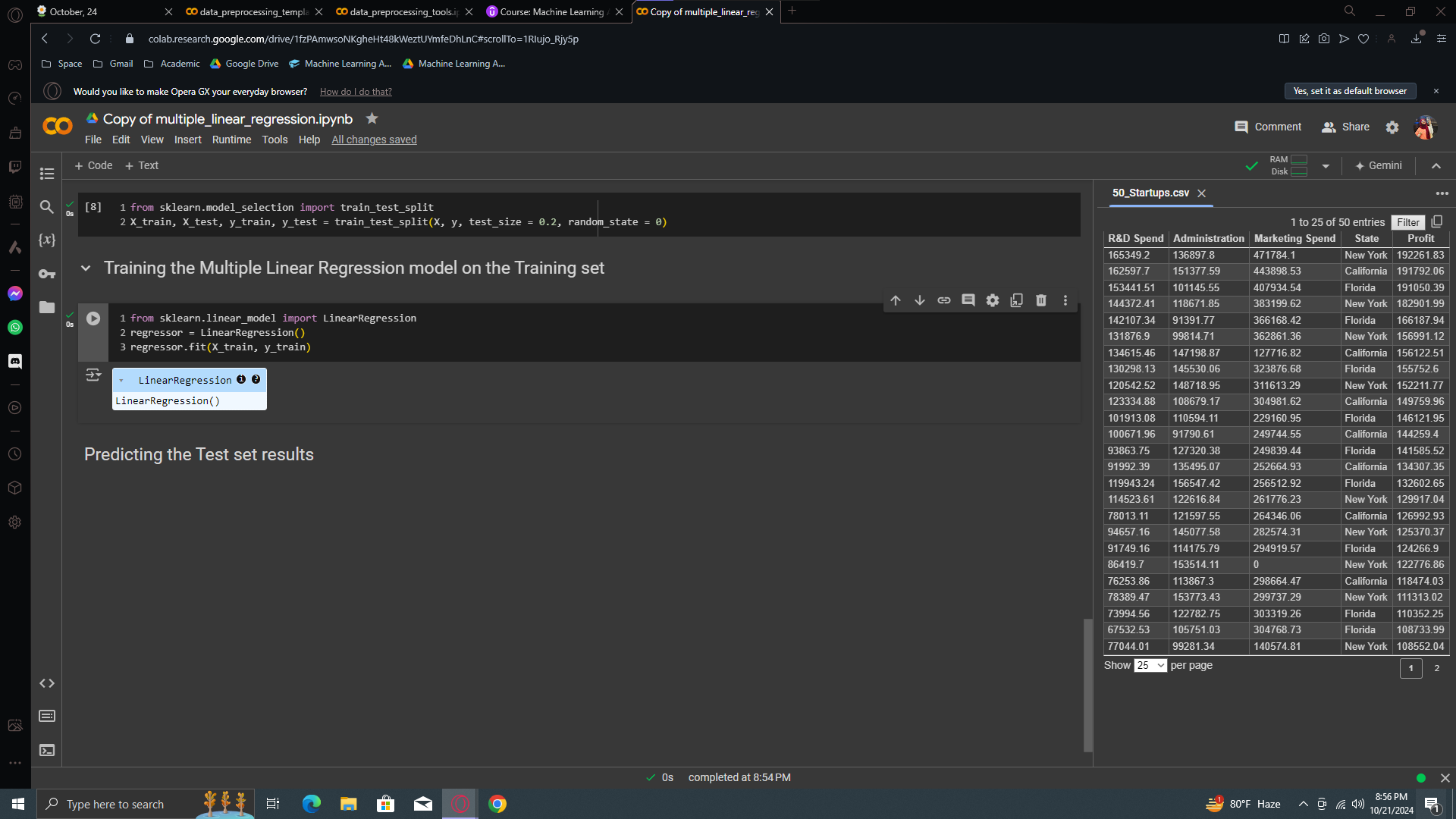
We now have a fully trained linear regression model on this dataset. It understands the correlations between different types of spending by 50 startups and their profit. Investors can use this model to predict the profit of new startups based on this information.

Thanks to this linear regression class, you don't have to worry about the dummy variable trap or selecting the best features. The class handles it all.

But, we need to understand something important. Unlike simple linear regression, we now have four features instead of one. We can't plot a graph like before because we would need a five-dimensional graph, which isn't possible for us to visualize. Instead, we'll display two vectors: one for the real profits from the test set and another for the predicted profits. The test set is 20% of the dataset, so with 50 observations, we'll have 10 samples. This allows us to compare the predicted profits with the real profits for each startup. And that's how we will evaluate our model. Later, you will learn about evaluation techniques to better measure the performance of your regression models with relevant metrics. For now, we'll see if our model performs well on new observations by comparing predictions to real results on the test set.

Predicting the Test set results

y_pred will be the vector of predicted profits in the test set. First, use the regressor object and apply the predict method with the test features. Next, call numpy and use the set_printoptions function to set the precision to 2, which will display two decimal places. Finally, use the concatenate function from numpy to combine vectors or arrays vertically or horizontally. In the parentheses, include y_pred, which is our vector of predicted profits. To arrange it vertically, use .reshape. This attribute allows you to reshape vectors or arrays. We need the number of elements in y_pred, which is the number of columns, so we use the len function here. Lastly, specify one, meaning you want to reshape your y_pred vector into an array with len(y_pred) rows and just one column.

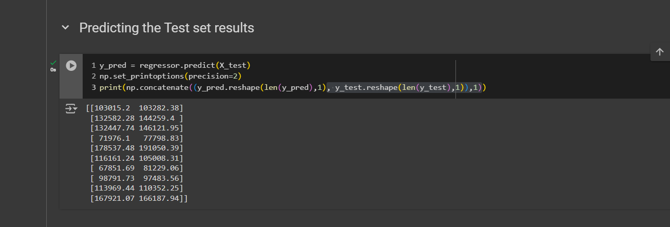
Next, copy-paste and put y_test instead of y_train. The axis here takes two values. 0 means we want to do a vertical concatenation and 1 means horizontal concatenation.

Now print and we can see 2 vectors here. On the left we have our predicted profits (y_pred) and on the right we have our vector of real profits [for 10 startups of the test set]. Now compare them. The first one is really good. prediction was 103015.2 and the actual one was 103282.38 - which is surely an amazing prediction.

Extra Content

Free BONUS exercise:

Question 1: How do I use my multiple linear regression model to make a single prediction, for example, the profit of a startup with R&D Spend = 160000, Administration Spend = 130000, Marketing Spend = 300000 and State = California?

Question 2: How do I get the final regression equation y = b0 + b1 x1 + b2 x2 + ... with the final values of the coefficients?

ans: https://colab.research.google.com/drive/1ABjLFzknByfU4-F4roa1hX36H3aZlu6J?usp=sharing

Enjoy the BONUS!

Machine Learning Chapter 2.2: Multiple Linear Regression

Table of contents