Machine Learning Chapter 2.4: Support Vector Regression (SVR)
 Fatima Jannet
Welcome to Machine Learning!
Support vector regression was created in the 90s by Vladimir Vapnik and his team at Bell Labs, which was known as AT&T Bell Labs back then. But for now, we'll focus just on linear regression. Let's get started!
SVR Intuition
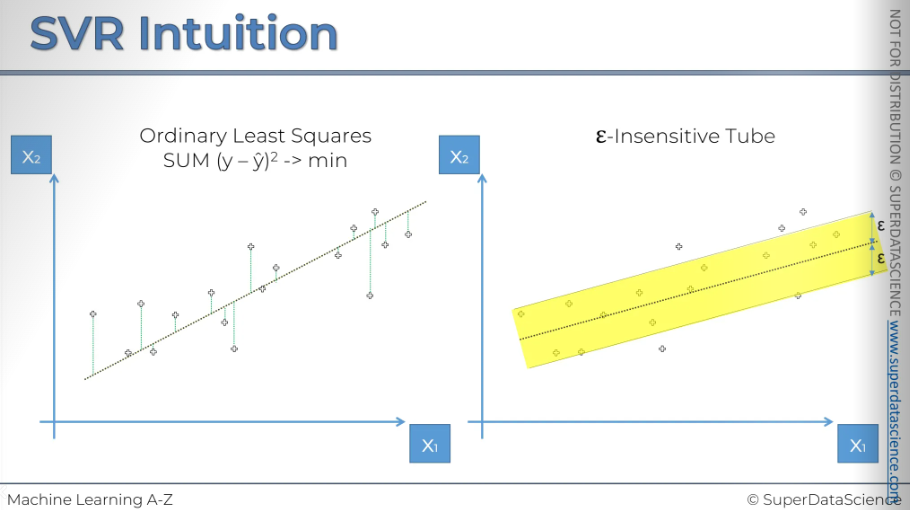
Here we have got two identical graphs to compare the Linear regression and SVR.
The random dots are positioned the same on both graphs. On the left, we have a linear regression model. We've discussed this before, but let's quickly review: We need to plot a line that goes through the data. To find this line, we use a method called the Ordinary Least Squares method. This method minimizes the distance, finding a path with the shortest distance to each dot.
Now, how does support vector regression (SVR) work? With SVR, instead of a line, you see a tube. The tube's purpose is to help minimize errors. This tube has a width called epsilon. It's known as the epsilon-insensitive tube. Any data point within this tube is disregarded as an error. This tube acts like a margin of error that we allow our model to have. Any error that falls within the tube's area is considered negligible.
Points that our outside of the tube are the error we have to take care of. Also we have to note their distance.
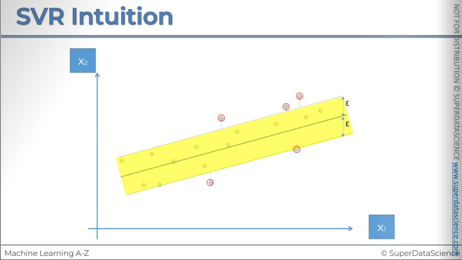
Every point on this plot is essentially a vector and can be represented by 2D vectors. The points outside the tube (marked in red) are called support vectors because they determine how the tube is formed. They support the structure of the tube, which is why they are called support vectors.
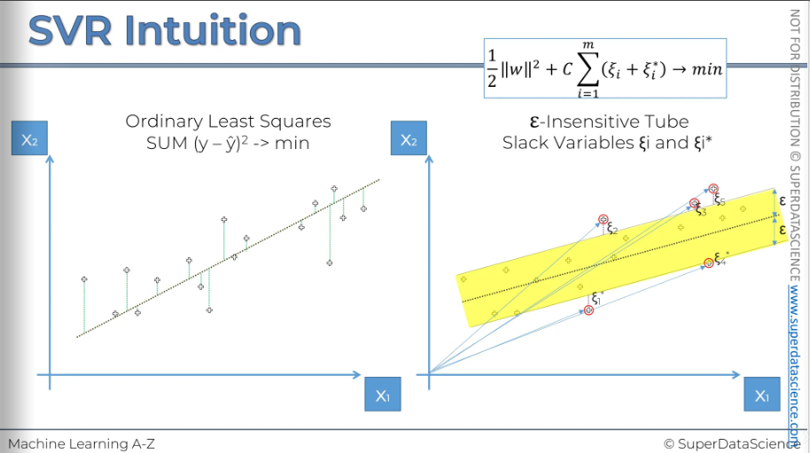
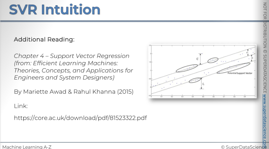
If you want to learn in-depth: Use the information given below
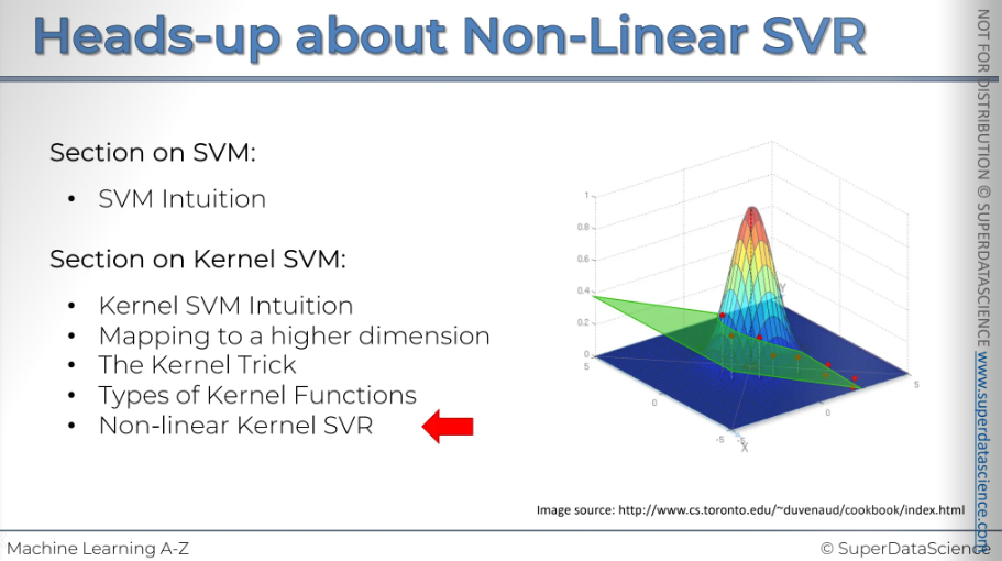
Non-linear SVR
Well, this is what you non linear SVR will look like in 3D. Earlier you saw the 2D version, now you are seeing the 3D version.
[I will write about the sections later, for now let’s stick with the codes]
SVR in Python
The model we are about to build is slightly more advanced than our previous ones.
Resources
Colab file: https://colab.research.google.com/drive/1BXw9jnH06_f_u7-B_dC-zGshce2fUsGZ
Data sheet: https://drive.google.com/file/d/1i9iYddj4Fwn5lDrXnPz7_y7TdvB62A1v/view
Data preprocessing template: https://colab.research.google.com/drive/17Rhvn-G597KS3p-Iztorermis__Mibcz
This is the exact same scenario we had in our Polynomial regression model, but this time we will use SVR to understand the correlation between position levels and the salaries. We just want to see if the support regression model performs better finding the salary of 160k/yr was true or not.
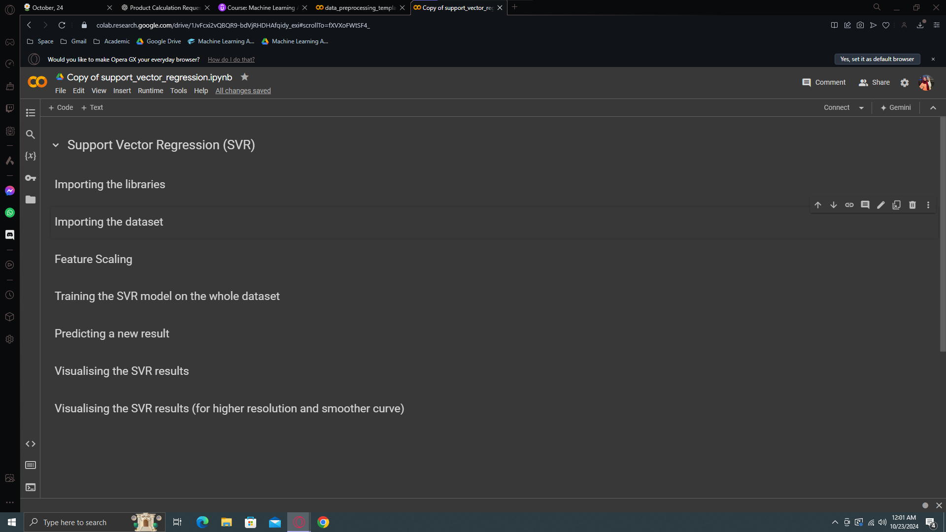
Code Implementation
Start with deleting all the code cells.
Importing Libraries
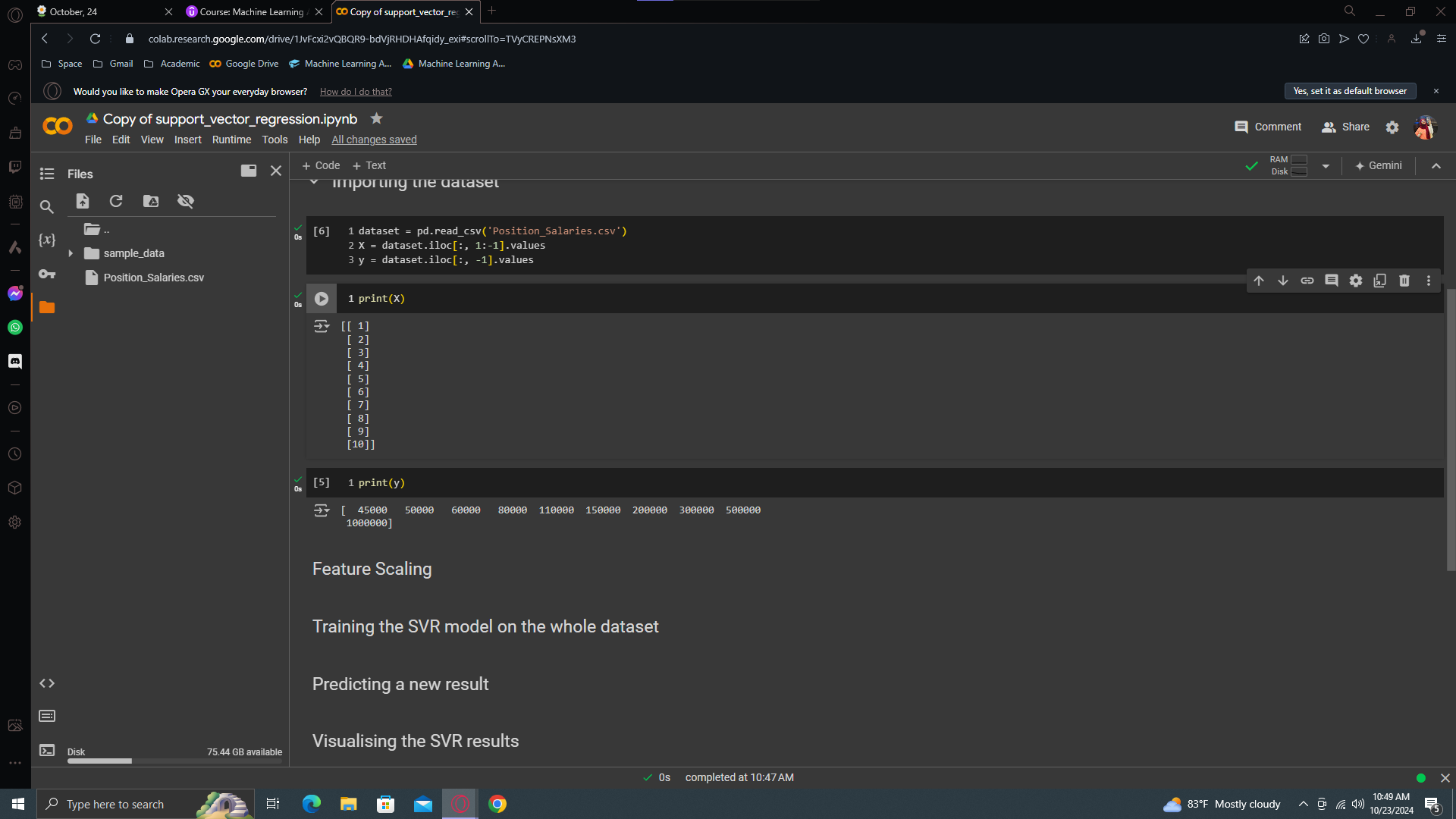
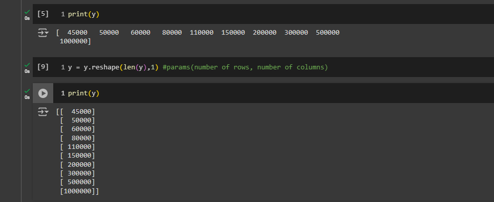
the standard scale class performs standardization, meaning feature scaling, and expects a 2D array as input. If you input a one-dimensional vector, it will return an error because it expects a 2D array. So, we need to transform this into a 2D array
Feature Scaling
First apply the feature scaling yo learnt from the 1st chapter of ML. We are going to modify the scaling section here
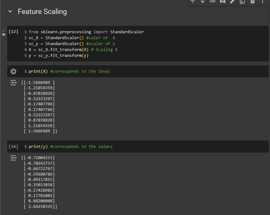
Look carefully, the values range from -1 to +3. Remember, in the data preprocessing section, I mentioned that standardization adjusts your values to range from -3 to +3.
Training the SVR model on the whole dataset
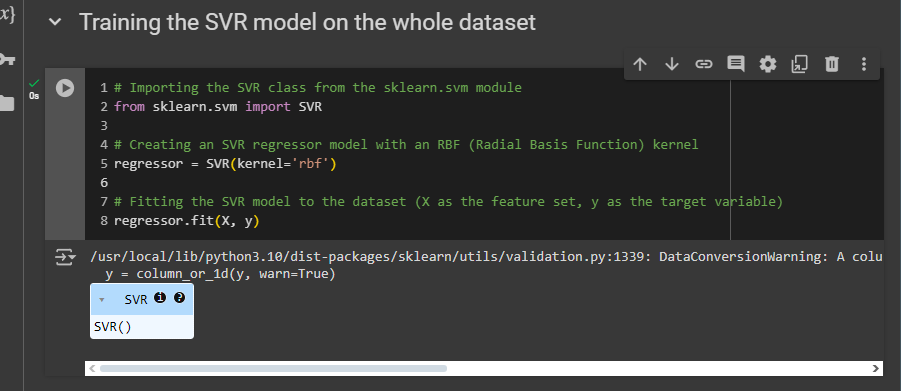
This is how you build and train an SVR model.
Predicting a new result

Visualising the SVR results
So we'll do it efficiently. We'll start from our polynomial regression implementation, including the visualization code at the end. We'll copy it. And then make changes according needs.
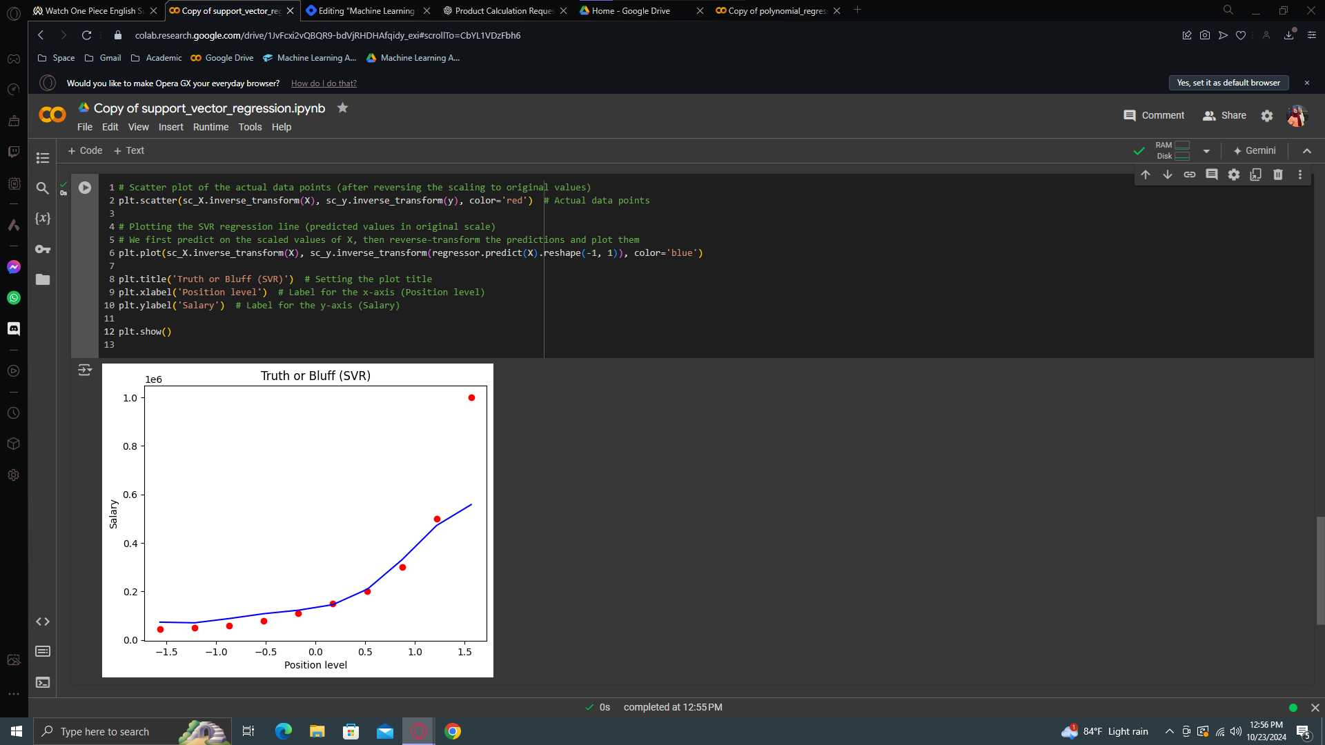
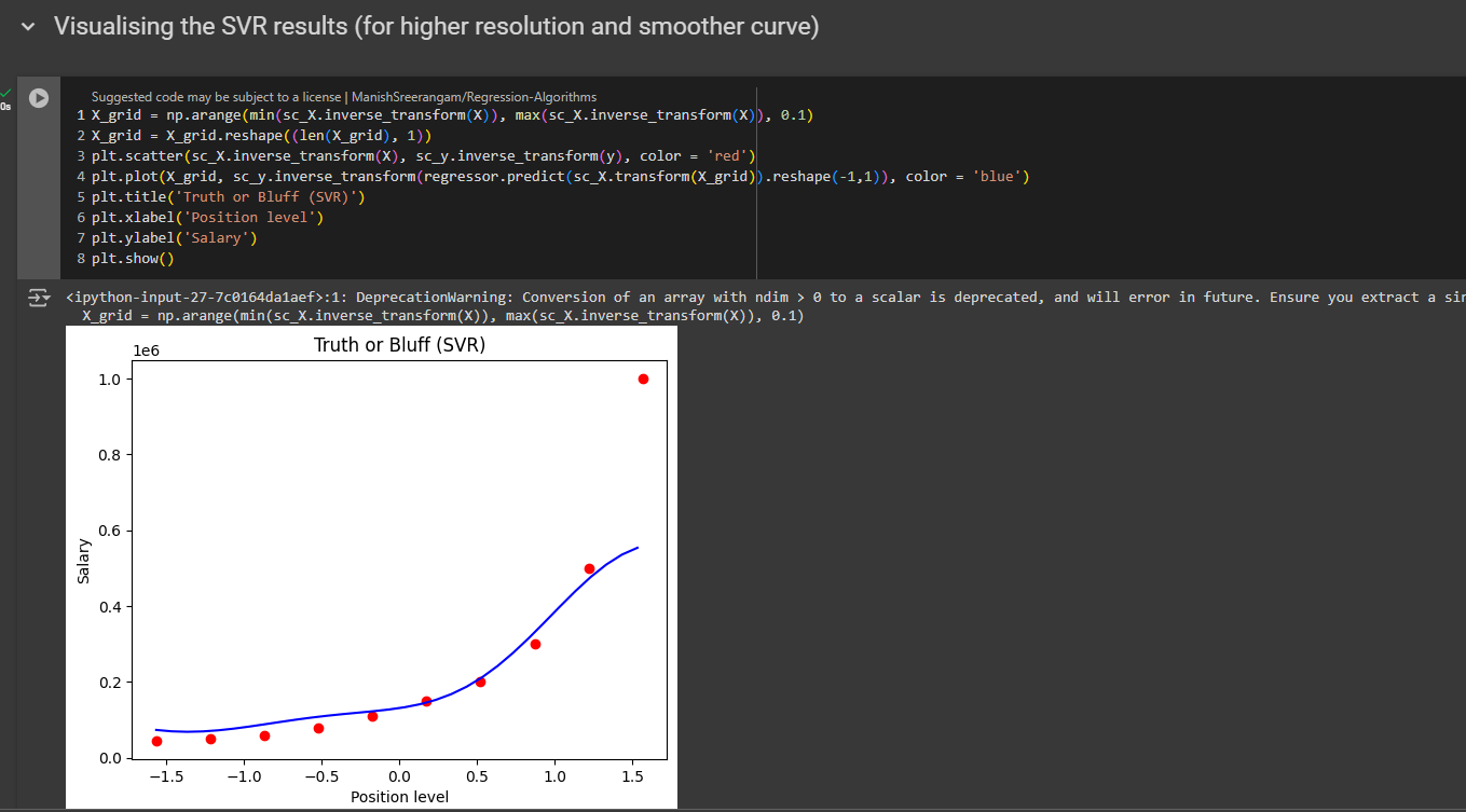
Visualising the SVR results (for higher resolution and smoother curve)
Again, go to your polynomial regression model, copy the code for smooth curve and paste and modify the code.
Poly:

SVR:
SVR Quiz
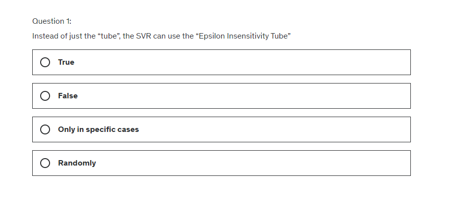
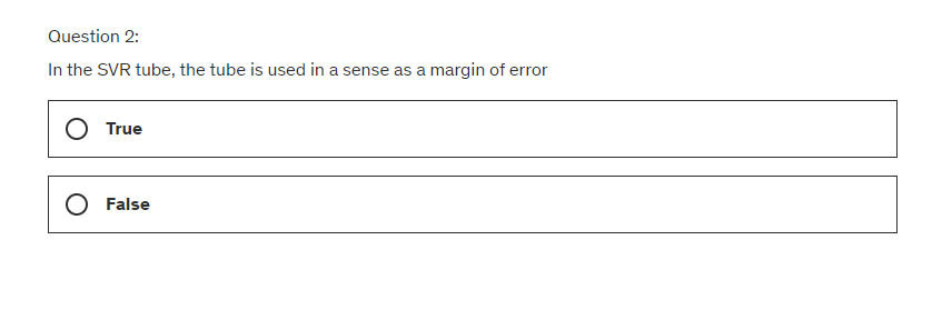
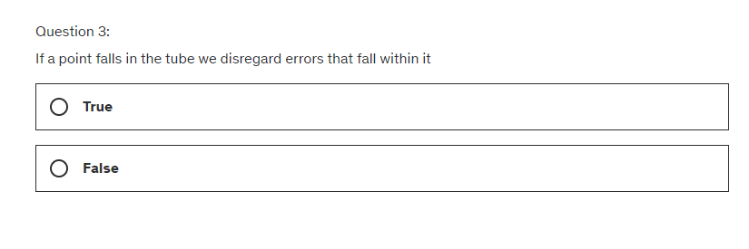
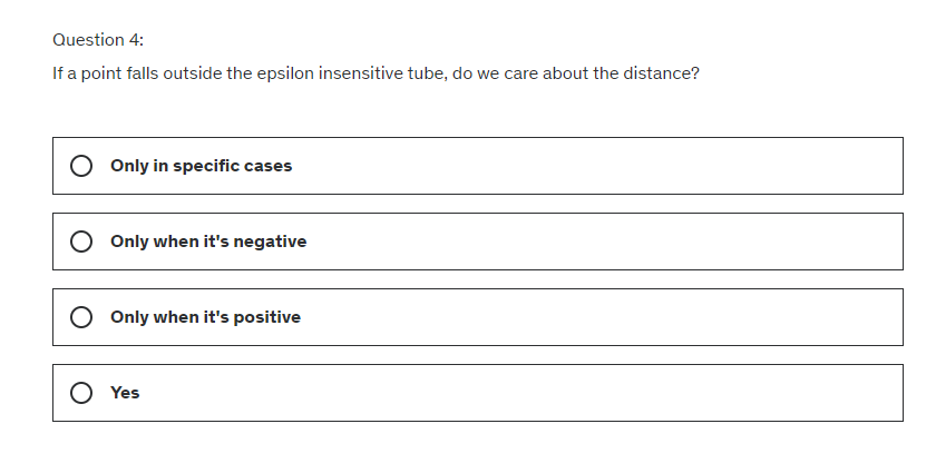
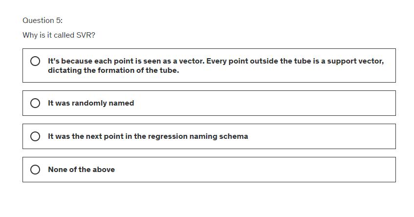
Answer: True, True, True, Yes, It’s because each point…..of the tube
Next blog is going to be on Decision tree regression.
Enjoy Machine Learning!
Subscribe to my newsletter
Read articles from Fatima Jannet directly inside your inbox. Subscribe to the newsletter, and don't miss out.
Written by
