This chapter explores the use of crypto trading simulators as a bridge between strategy development and live trading. Many exchanges, including Binance, offer simulated trading environments that replicate market dynamics and exchange rules. For quantitative traders, it’s advisable to first develop and refine strategies in a simulated environment. Once the strategy proves successful, it can be deployed for live trading by replacing API endpoints and authentication credentials.

We’ll leverage DolphinDB’s httpClient plugin for interacting with Binance’s private API, including account position queries for spot and futures, order placement, status checks, and cancellation. To illustrate practical applications, we present two strategy implementations: TWAP (Time-Weighted Average Price) and pair trading. This section is focused on the TWAP strategy.

Download the whole whitepaper here: Cryptocurrency Solutions — Dolphindb

6.1 Functions for Interacting with Binance’s API

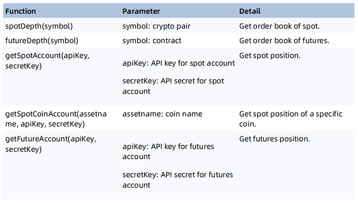
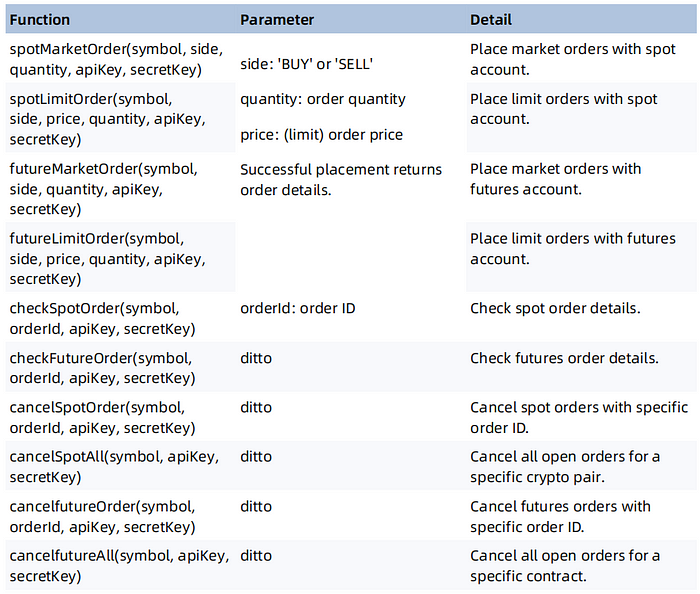
DolphinDB has developed a suite of functions to interact with Binance’s API. These functions streamline the process of making requests to Binance, enabling seamless integration of trading operations within the DolphinDB environment. To access these capabilities, simply load the liveTradingAPI.dos into your DolphinDB session. The table below presents an overview of the supported functions. Detailed description can be referred to Appendix.

Table 6–1 List of Functions for Interacting with Binance’s API

6.2 TWAP Strategy

TWAP (Time-Weighted Average Price) is a widely used algorithmic trading approach designed to execute large orders. This strategy works by systematically dividing a large order into smaller, equal-sized portions and executing them at regular intervals over a predetermined timeframe, thus achieving a price close to the average over a specified period. TWAP spreads the trading quantity evenly across time, reducing the likelihood of causing significant price movements that often result from large, single-block trades.

When implementing a TWAP strategy, traders can fine-tune several key parameters:

Trading Period: The timeframe for order execution, setting both start and end times.
Total Order Quantity: The overall quantity of the asset to be traded.
Time Interval: The time interval to execute partial orders. This divides the total trading period into equal segments.
Order Size per Interval: The quantity of assets to be traded in each time interval.
Slippage Tolerance: The acceptable range of price deviation from the expected execution price.
Price Limits: The upper and lower bounds for execution prices.

6.2.1 Workflow

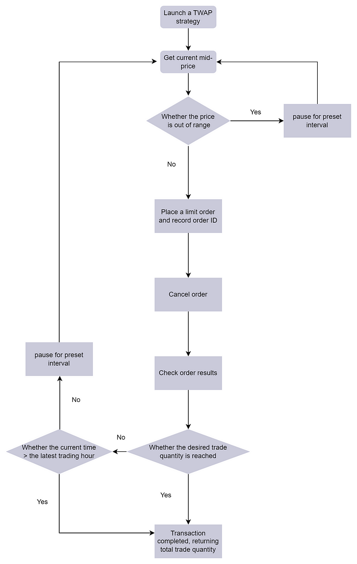
The TWAP strategy implementation revolves around an iterative process that executes several key steps: place or cancel a sub-order; update order status and trade details; pause for a predetermined interval. This loop continues until either the desired total quantity is reached or the specified time range expires, at which point the strategy concludes and reports the total executed quantity.

For each individual sub-order, the process begins by obtaining the current mid market price. The strategy then adjusts the order price based on the preset slippage tolerance. If the calculated price falls outside the predefined price slippage, the strategy pauses for the set interval before reassessing market conditions. Once the price aligns with the strategy’s parameters, it proceeds with placing the sub-order.

The following figure shows the workflow of the TWAP strategy.

Figure 6–1 Workflow of the TWAP Strategy

6.2.2 Key Functions for Order Execution

To implement our TWAP strategy effectively, we need to address two key aspects: market data access and order execution.

For market data access, we utilize the methods outlined in Chapter 2. To simplify this demonstration, we’ll be using DolphinDB’s httpClient plugin to fetch real-time quotes.

Regarding order execution, we prioritize performance and high availability. To allow for real-time updates and retrieval of order information and quick total quantity calculations, we adopt a persisted stream table that serves as a cache for order statuses and related info.

Creating a Persisted Stream Table

Create a persisted stream table “ordersDetail“ to store order info including labels, crypto pairs, update times, IDs, prices, order quantities, trade quantites, statuses, types and directions.

colNames = `label`symbol`updatetime`orderId`price`origQty
           `executedQty`status`type`side
colTypes = [STRING,SYMBOL, TIMESTAMP, INT, DECIMAL128(18), 
            DECIMAL128(18), DECIMAL128(18), STRING, STRING, STRING]
enableTableShareAndPersistence(table=streamTable(100000:0, 
                               colNames, colTypes), tableName=`ordersDetail, 
                               cacheSize=1200)

Placing Orders

In the TWAP strategy, when a sub-order is successfully placed, the exchange responds with related order information. This data is immediately captured and appended to the “ordersDetail” table.

The function is defined as follows:

def putOrderRecordDetails(labelName,symbol,side,price,
                          eachQty,sapi_key,sapi_secret){
    slimit = spotLimitOrder(symbol,side,price,eachQty,sapi_key,sapi_secret)
    openOrderTable = table(labelName as label, slimit['symbol'] as symbol, 
                     now() as updatetime, 
                     slimit['orderId'] as orderId, 
                     slimit['price']$DECIMAL128(18) as price, 
                     slimit['origQty']$DECIMAL128(18) as origQty, 
                     slimit['executedQty']$DECIMAL128(18) as executedQty, 
                     slimit['status'] as status, 
                     slimit['type'] as type, 
                     slimit['side'] as side)
                     ordersDetail.append!(openOrderTable)
}

For optimal execution, we initiate orders at prices slightly less favorable, i.e., buy orders with a price above the mid price, or sell orders with a price below the mid price. For instance, if the mid-market price is 100.0, we might place a sell order at 99.0. While technically a limit order, this pricing strategy typically ensures rapid execution under normal market conditions.

Canceling Orders

To adapt to potential market fluctuations or brief periods of illiquidity, we’ve incorporated an order cancellation mechanism. Define the function to query the “ordersDetail” table for orders with a “NEW” status and identify the corresponding order IDs that were targeted for cancellation. For successfully canceled orders, we update their status in the “ordersDetail” table from “NEW” to “CANCELED”.

def cancelOrders(labelName,symbol,sapi_key,sapi_secret){
    lastOrdersDetial = select last(label) as label, orderId,
    last(status) as status from ordersDetail group by orderID
    toCancelID = exec orderId from lastOrdersDetial 
                 where label = labelName and status = 'NEW'
    for(ID in toCancelID){cancelSpotOrder(symbol, ID, sapi_key,sapi_secret)}
}

Checking Orders

The checkOrders function retrieves order information and inserts the latest order details into the stream table "ordersDetail”.

def checkOrders(labelName,symbol,sapi_key,sapi_secret){
    lastOrdersDetial = select last(label) as label, orderId,
    last(status) as status from ordersDetail group by orderID
    toCheckID = exec orderId from lastOrdersDetial 
                where label = labelName and status = 'NEW'
    for(ID in toCheckID){
        cOrder = checkSpotOrder(symbol,ID,sapi_key,sapi_secret)
        checkedOrderTable = table(labelName as label, cOrder['symbol'] as symbol, 
                                  now() as updatetime, 
        cOrder['orderId'] as orderId, cOrder['price']$DECIMAL128(18) as price, 
        cOrder['origQty']$DECIMAL128(18) as origQty, 
        cOrder['executedQty']$DECIMAL128(18) as executedQty, 
        cOrder['status'] as status, 
        cOrder['type'] as type, cOrder['side'] as side)
        ordersDetail.append!(checkedOrderTable)
    }
}

Calculating Total Trade Quantity

To maintain a comprehensive view of our TWAP strategy, we continuously monitor the overall trade quantity. This crucial metric is derived from the data stored in our “ordersDetail” table.

def calTradeQty(labelName){
    tradedQty = select last(label) as label, orderId, last(symbol) as symbol, 
                last(price) as price, last(status) as status,
                last(executedQty) as executedQty 
                from ordersDetail group by orderID
    sumQty = exec sum(executedQty) from tradedQty where label = labelName
    return sumQty
}

6.2.3 Core Implementation

The core implementation of our TWAP strategy revolves around a loop, managing order placement, cancellation, and trade quantity tracking. Upon completion of the loop, the function outputs the total quantity of trades executed (lines 31–32).

Within each iteration, the loop first retrieves the mid-market price and calculates the order price based on preset slippage (priceSlippage) and trading direction (side). This price is then validated against predefined tolerance levels (priceTolerance). If the calculated price falls outside these bounds (exceeding the upper limit for buy orders or falling below the lower limit for sell orders), the process pauses briefly (gaptime) before proceeding to the next cycle.

The heart of the loop (lines 20–25) handles the core order management functions. It places new orders (with price, side, and eachQty), cancels open orders, and updates their statuses. The trade quantity is calculated and returned.

The loop’s exit conditions are evaluated in lines 26–28. The process terminates if either the total executed quantity (sumQty) reaches the target (totalQty) or the current time exceeds the specified end time (endtime). If neither condition is met, the loop pauses for a set interval (gaptime) before initiating the next cycle.

def twapSpotTool(labelName, symbol, side,priceTolerance, 
                 priceSlippage, totalQty, eachQty, gaptime, 
                 endtime, apiKey, secretKey){
    do{
    depth = spotDepth(symbol)
    if(side == 'BUY'){
        price = (depth['bids'][0][0]$DOUBLE+depth['asks'][0][0]$DOUBLE)/2
        price = ((1+priceSlippage)*price)$DECIMAL128(2)
        if(price > priceTolerance){
            sleep(1000*gaptime)
            continue}
    }
    else{
        price = (depth['bids'][0][0]$DOUBLE+depth['asks'][0][0]$DOUBLE)/2
        price = ((1-priceSlippage)*price)$DECIMAL128(2)
        if(price < priceTolerance){
            sleep(1000*gaptime)
            continue}
    }
    slimit = spotLimitOrder(symbol,side,price,eachQty,apiKey,secretKey)
    putOrderRecordDetails(labelName,symbol,side,price,eachQty,apiKey,secretKey)
    cancelOrders(labelName,symbol,apiKey,secretKey)
    checkOrders(labelName,symbol,apiKey,secretKey)
    sumQty = calTradeQty(labelName)
    print(sumQty$DECIMAL128(2))
    if(sumQty>=totalQty){break}
    if(now()>endtime){break}
    sleep(1000*gaptime)
    }
    while(1)
    sumQty = calTradeQty(labelName)
    print('TotalTradeQTY:',sumQty)
}

6.2.4 Scheduled Execution

DolphinDB’s built-in function scheduleJob allows users to automate the execution of TWAP strategy, twapSpotTool, at preset times or intervals.

Consider the following scenario: We have a TWAP strategy script twap.dos that we want to execute at a specific time — July 31, 2024, at 03:30 AM. To schedule this execution in DolphinDB, use the following script:

scheduleJob(jobId=`once, jobDesc="Twap Job 1", 
            jobFunc=run{"twap.dos"}, scheduleTime=03:30m, 
            startDate=2024.07.31, 
            endDate=2024.08.01, 
            frequency='M', days=1)

6.2.5 Example

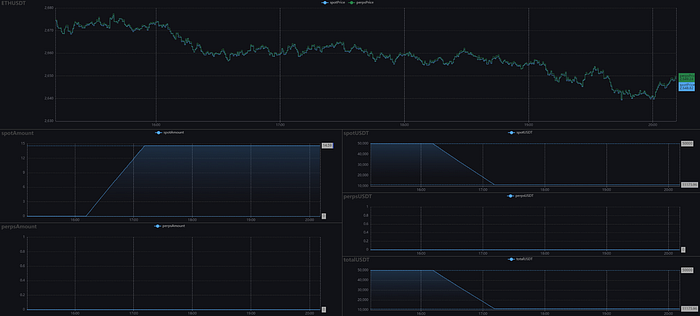
The following is an example that runs twapSpotTool at 2024.07.01 16:31:30.

twapSpotTool(labelName='TWAP_SELL_ETHUSDT_EXAMPLE', symbol='ETHUSDT', side='BUY',
priceTolerance=4000, priceSlippage=0.01, totalQty=10, eachQty=0.2, gaptime=2, 
endtime = 2024.07.01 23:00:00, apiKey = sapi_key,secretKey = sapi_secret)

You can observe that the USDT balance in the spot account has decreased while the ETH holdings have increased, aligning perfectly with the intended outcome of the strategy.

Figure 6–2 Visualization of TWAP Strategy’s Result

In the above section we introduced implementations of TWAP strategies. Stay tuned and explore pair trading strategy in the upcoming section with us!

Crypto Trading Simulation for Live Market Execution (Trading with TWAP Strategy)