All about Pandas and Numpy
 Ashmit Kanti
Numpy
NumPy is a library for the Python programming language, adding support for large, multi-dimensional arrays and matrices, along with a large collection of high-level mathematical functions to operate on these arrays.
Guide to Numpy: -
NumPy user guide — NumPy v2.2.dev0 Manual
In order to add this library, we use the import function i.e.: -
import numpy as np
Arrays
Suppose, you have a list: -
list_1 = [50,60,70,80,90,100]
You can convert it into array: -
my_numpy_array = np.array(list_1)
my_numpy_array

#Output: - array([ 50,  60,  70,  80,  90, 100])
So, we have an array here.
Difference between an array and list basically is that in an Array, all the items are of the same type and the size of array is set when we create an Array (in most languages it is set but for some reason it is not set in Python 😅*)*.
Suppose, you host a site and when users sign in, you don’t want some of the usernames to be numbers or signs or anything, this is where arrays are used as they will only take a single data type here.
We can create multi dimensional array too.
my_multi_dimensional_array = np.array([[1,2,3], [4,5,6]])
my_multi_dimensional_array

#Output: - array([[1, 2, 3],
#       [4, 5, 6]])
Suppose, we want to make an array but only specify the number of values we want but not the value i.e. randomly generate the value, then we use Rand function.
# "rand()" uniform distribution between 0 and 1

x = np.random.rand(10)
x

#Output: - array([0.94741471, 0.49486095, 0.22979935, 0.85434421, 0.46749842,
#       0.3037954 , 0.21403418, 0.07955939, 0.25948629, 0.14459976])
Suppose, now you want to built a multi dimensional array e.g. $3 \times 3$ but want each number to be random too.
# you can create a matrix of random number as well
y = np.random.rand(3,3)
y

#Output: - array([[0.53203366, 0.83228422, 0.80424709],
                    #       [0.32818021, 0.82824937, 0.07370119],
                    #       [0.63439739, 0.9397671 , 0.39533399]])
Leave array for a moment 🙂, suppose we want to get a random integer between $1$ and $50$, we can easily do that too: -
x = np.random.randint(1,50)
x

#Output: - 22
Suppose, you wanna generate 15 different integers at the same time, you specify it in the 3rd space in bracket.
x = np.random.randint(1,50, 15)
x

#Output: - array([ 9, 31,  3,  1, 13, 17, 34, 21, 27, 46, 11, 12, 32, 49,  3])
#We get an array of 15 randomly generated integers
Suppose, now you want an array which has all the elements from 1 to 20 i.e. counting from 1 to 20, this is where np.arange comes in handy.
x = np.arange(1,20)

#Output: - array([ 1,  2,  3,  4,  5,  6,  7,  8,  9, 10, 11, 12, 13, 14, 15, 16, 17,
#                               18, 19])
and I we wanna add order of how they are generated, we can use the 3rd position in the bracket for that.
x = np.arange(1,20,2)

#Output: - array([ 1,  3,  5,  7,  9, 11, 13, 15, 17, 19])
#Each numbers gapped by 2
Suppose, you wanna make an identity array i.e. an array which has all the elements as zero except the diagonal elements as 1, we could make it possible using eye
x = np.eye(7)
x
#Output: - array([[1., 0., 0., 0., 0., 0., 0.],
                        #     [0., 1., 0., 0., 0., 0., 0.],
                        #     [0., 0., 1., 0., 0., 0., 0.],
                        #     [0., 0., 0., 1., 0., 0., 0.],
                        #     [0., 0., 0., 0., 1., 0., 0.],
                        #     [0., 0., 0., 0., 0., 1., 0.],
                        #     [0., 0., 0., 0., 0., 0., 1.]])
# It is a 7X7 identity array
If you wanna create an array which has all the elements as 1, use the ones function.
j = np.ones((3,7)) #Just be careful of the brackets here. It can also be like((3,7), dtype=int) i.e. datatype could also be declared.
j

#Output: - array([[1., 1., 1., 1., 1., 1., 1.],
                           #[1., 1., 1., 1., 1., 1., 1.],
                           #[1., 1., 1., 1., 1., 1., 1.]])
To do the same for zero instead of one, use zeros function.
We can effectively add 2 arrays too.
x = np.arange(1,10)
#Output: - x = array([1, 2, 3, 4, 5, 6, 7, 8, 9])

y = np.arange(1,10)
#Output: - y = array([1, 2, 3, 4, 5, 6, 7, 8, 9])

sum = x + y
#Output: - Sum: - array([ 2,  4,  6,  8, 10, 12, 14, 16, 18])
You can also square an array using ** i.e. all the elements in the array will be squared.
x = np.arange(1,10)
#Output: - x = array([1, 2, 3, 4, 5, 6, 7, 8, 9])

h = x**2
h
#Output: - array([ 1,  4,  9, 16, 25, 36, 49, 64, 81])
If you ever wanna create a $m \times n$ array with all the numbers random or between some range: -
x = np.random.randint(1,35,[4,4])  #A 4x4 matrix with all the random numbers in the range of 1 to 35
#Output: - array([[15, 21, 16, 33],
                           #[19,  4, 14, 27],
                           #[31,  3,  8, 23],
                           #[17, 17,  8, 18]])
Suppose, we wanna access any row of the array, then we need to call them by index number too.
Suppose, we have an array: -
ary = np.array([[15, 21, 16, 33],  #Index Number: - 0
                                [19,  4, 14, 27],  # Index Number: - 1
                                [31,  3,  8, 23],  # Index Number: - 2
                                [17, 17,  8, 18]]) # Index Number: - 3
In order to access any specific row: -
ary[1]

# Output: - array([19, 4, 14,  27])
What if you wanna access a particular element in a multi dimensional array, we use 2 square brackets adjacent to the name of matrix, one for the row, other for the column.
ary[1][2] #First bracket specifies the row number by its index, the second bracket specific the column number of that row
#Output: - 14
Suppose we create a new array with the dimensions of $4 \times 5$ filled with random integers from 1 to 10 i.e.: -
ble = np.random.randint(1,10,(4,5))

#Output: - array([[2, 3, 6, 4, 1],
                           #[9, 9, 5, 1, 2],
                           #[3, 6, 1, 1, 6],
                           #[8, 5, 7, 2, 1]])
Suppose, we now wanna filter out the elements, e.g. want to filter out only that elements which are greater than $7$. In order to do this, we will have to create a new array which will have effect on the the original array.
new_array = ble[ble > 7]

#Output: - array([9, 9, 8])
We can see that there were only 3 occurrences where we had the output greater than 7 and it is shown in here.
Take example the our array ble , what if we want to replace all the odd elements in the array by 2, then the code would look like: -
ble[ble % 2 != 0] = 2

#Output: - array([[2, 2, 6, 4, 2],
                           #[2, 2, 2, 2, 2],
                           #[2, 6, 2, 2, 6],
                           #[8, 2, 2, 2, 2]])
The command is like change ble , where is ble is division by 2 doesn’t give the result as $0$, replace by $2$.
Pandas
You can think of Pandas as Microsoft Excel of Python 🐍
At first import pandas as a library: -
import pandas as pd
Suppose, you wanna create this table: -
| Name | Standard |
| Ashmit | 12 |
| Kavya | 13 |
In order to create this table in python, the code will look like: -
student = pd.DataFrame({'Name':['Ashmit', 'Kavya'], 'Standard':[12,13]})
First and foremost, we name the table student and then we declare pd i.e. pandas to be used and then we use the function DataFrame (DataFrame is case sensitive, dataframe ❌, DataFrame ✅) to put the data in a tabular form and then we enter () and inside these, we enter { } and define the heading of the column in single inverted commas i.e. ‘ ‘ such as how name is defined here and then we use : to indicate towards the data present in the body of these columns, the data of the body is stored in [ ] . Rest of the queries will be most probably solved observing the example.
The output looks like: -

Suppose we’re reading a webpage and come across some tables: -

what if we wanna get these tables imported into python, this is where pd.read_hmtl gets into work.
import pandas as pd

outside_table = pd.read_html('<https://www.livingin-canada.com/house-prices-canada.html>')
print(outside_table)
and we get the result as: -
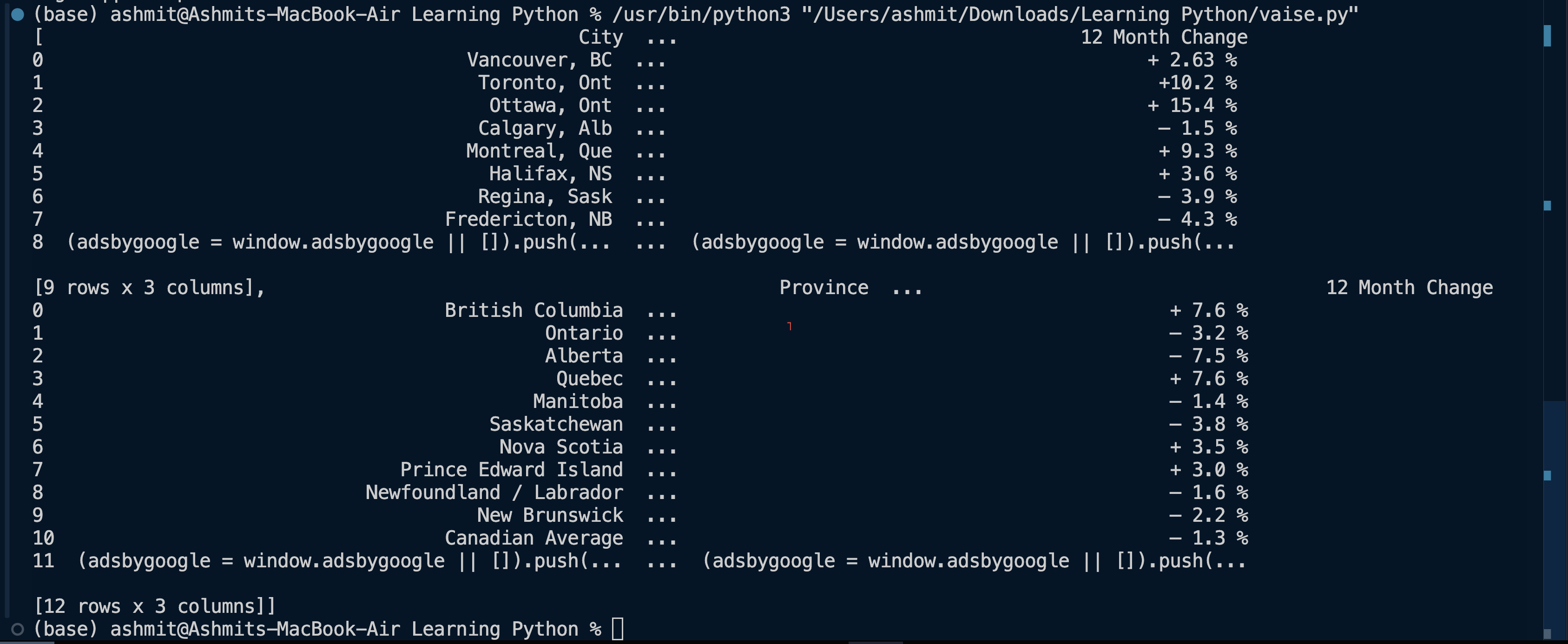
We. can see that both the tables were successfully imported into python.
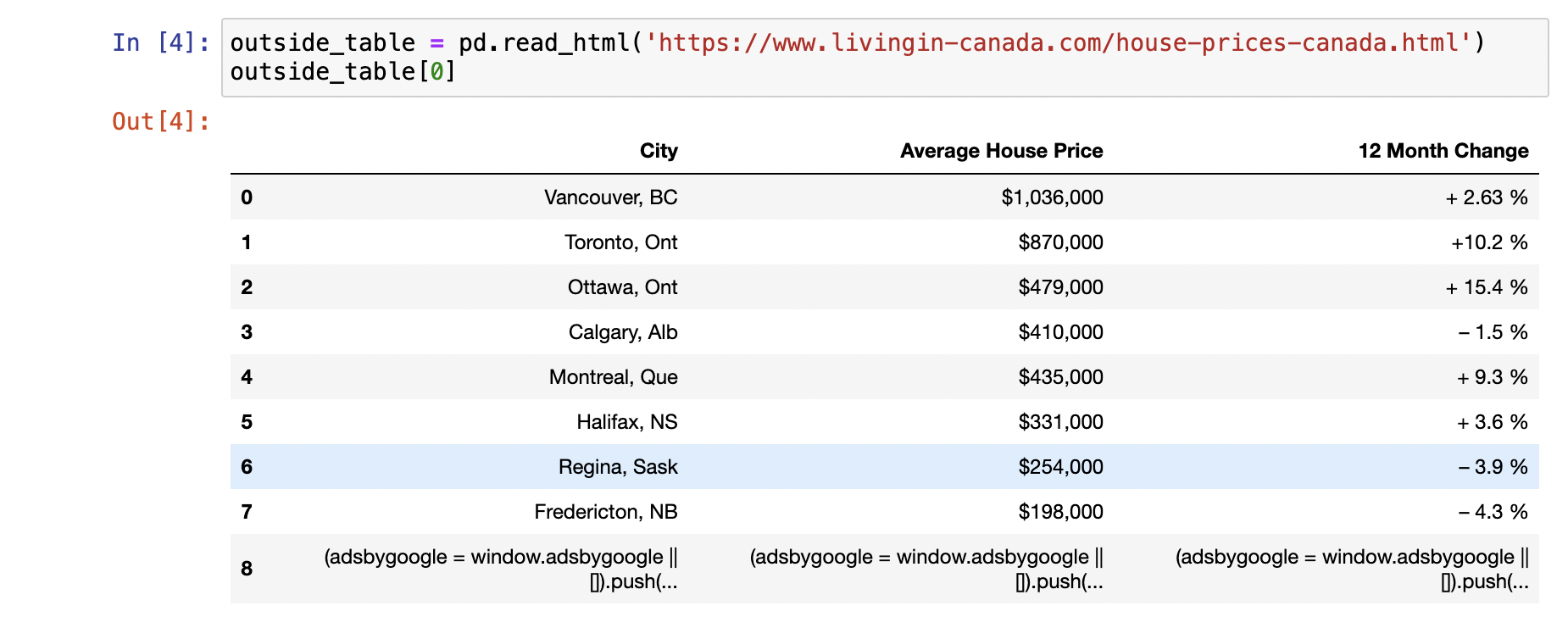
Now, we can clearly see that they have more than one tables on a single page, if we only need to print a single table at a time, we will have to specify it, each table differ by its index number, the first table will be accessed by index number $0$, the second table will be accessed by index number $1$, e.g the first table is accessed as follows: -
Suppose, we have a table: -
studentss = pd.DataFrame({'Name':['Ashmit', 'Kavya', 'Ankita', 'Maaz'], 'Standard':[12,13,19,9]})
The table is like: -
| Name | Standard |
| Ashmit | 12 |
| Kavya | 13 |
| Ankita | 19 |
| Maaz | 9 |
Suppose, I wanna filter out of contents of table e.g. what I only want the students which have standards greater than 12.
seniors = studentss[ studentss['Standard'] > 12 ]
Output: -
| Name | Standard |
| Kavya | 13 |
| Ankita | 19 |
In order to delete a certain column in python, use the del , e.g. here we wanna delete the Standard column: -
del studentss['Standard']
Output: -
| Name |
| Kavya |
| Ankita |
Applying functions in Tables too
Suppose we have a table: -
bank_client_df = pd.DataFrame({'Bank client ID':[111, 222, 333, 444],
                               'Bank Client Name':['Chanel', 'Steve', 'Mitch', 'Ryan'],
                               'Net worth [$]':[3500, 29000, 10000, 2000],
                               'Years with bank':[3, 4, 9, 5]})
bank_client_df

Suppose, there is an event of some sort and you want to Thank the customers for being loyal and give them each a $1000 i.e. add $1000 to their net worth then you can create a function too that does operations on the data too.
def give_bonus(balance):
    return balance + 1000
and then we apply the function: -
bank_client_df['Net worth [$]'].apply(give_bonus)
Here, we at first specify the column and then we tell the system to apply the specific function.
Take the table as previously used, suppose, we want to sort out the items now, e.g. what if we want the people to be sorted by their bank balance i.e. placed from lower bank balance to higher bank balance.
bank_client_df.sort_values(by = 'Net worth [$]')

All of is done is good, but all this change is temporary i.e. none of this change is made to the real table in memory i.e. if you print the real table again, you will realise that there is practically no change done to the table, for this while applying these types of commands, you need to use inplace = True clause in any statement and it will work like a charm.
bank_client_df.sort_values(by = 'Net worth [$]', inplace = True)
and if we check the table again, the changes have been made to the memory.
Suppose, we have a table
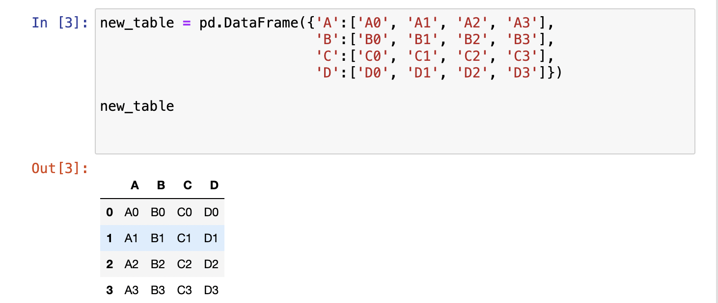
and we create another 2 tables just like that: -
new_table2 = pd.DataFrame({'A':['A4', 'A5', 'A6', 'A7'],
                          'B':['B4', 'B5', 'B6', 'B7'],
                          'C':['C4', 'C5', 'C6', 'C7'],
                          'D':['D4', 'D5', 'D6', 'D7']})

new_table3 = pd.DataFrame({'A':['A8', 'A9', 'A10', 'A11'],
                          'B':['B8', 'B9', 'B10', 'B11'],
                          'C':['C8', 'C9', 'C10', 'C11'],
                          'D':['D8', 'D9', 'D10', 'D11']})
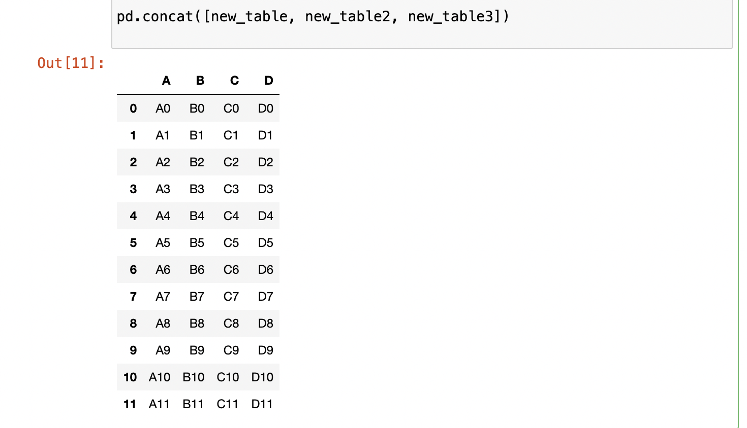
and in order to concatenate these 3 tables, we need to use pd.concat clause, where we mention the tables, we need to concatenate
pd.concat([new_table, new_table2, new_table3])
and we get the result as: -
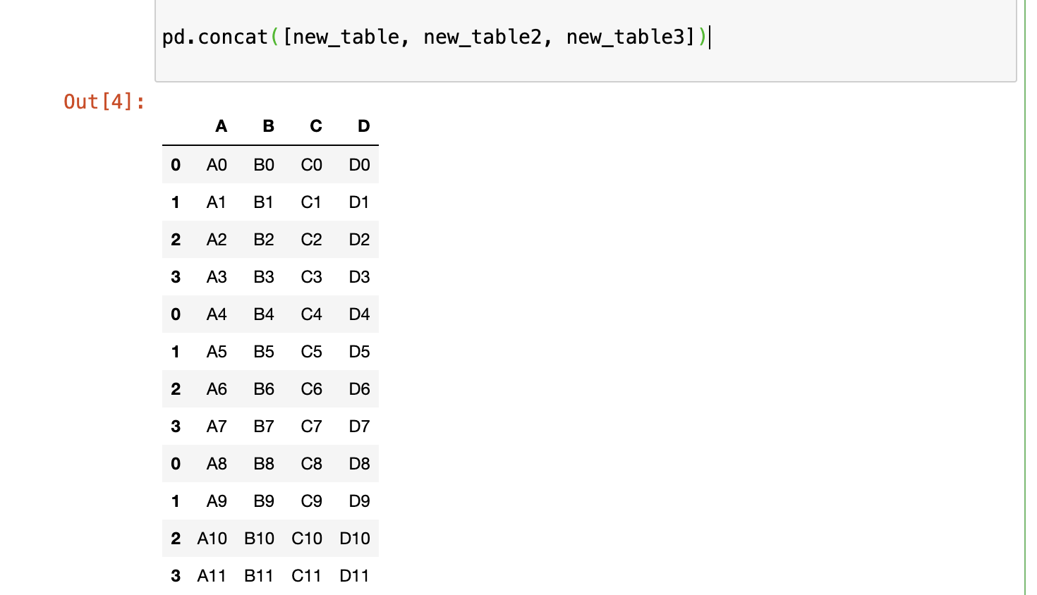
but, here we account a slight problem i.e. see in the first column, the numbers repeat again and again from 0 to 3, so in this case, we need to take care of the what known as index for the table and assign it in each table.
#The code for first table is something like: -
new_table = pd.DataFrame({'A':['A0', 'A1', 'A2', 'A3'],
                          'B':['B0', 'B1', 'B2', 'B3'],
                          'C':['C0', 'C1', 'C2', 'C3'],
                          'D':['D0', 'D1', 'D2', 'D3']}
                        index = [0,1,2,3])

# The addition to table 2: -
index = [4,5,6,7])

# The addition to table 3: -
index = [8,9,10,11])
and now the results look stunning: -
This is what it is all about Pandas and Numpy as whole and if you read the whole thing, I don’t think you would need more help, but if you ever do, just get in contact with me, I will make sure to help you with all the resources I have.
Thanks for your time and attention.
Regards,
Ashmit Kanti
Subscribe to my newsletter
Read articles from Ashmit Kanti directly inside your inbox. Subscribe to the newsletter, and don't miss out.
Written by