print(result) "Part 4 of NotADev"

Introducing Machine Learning

Now that the data was enriched with technical indicators and lag features, it was time to build a predictive model to forecast stock movements.

Building the Predictive Model

The AI assistant suggested using XGBoost, a powerful and efficient gradient boosting algorithm that's well-suited for tabular data.

What is XGBoost in Machine Learning?

XGBoost, or eXtreme Gradient Boosting, is a XGBoost algorithm in machine learning algorithm under ensemble learning. It is trendy for supervised learning tasks, such as regression and classification. XGBoost builds a predictive model by combining the predictions of multiple individual models, often decision trees, in an iterative manner.

The algorithm works by sequentially adding weak learners to the ensemble, with each new learner focusing on correcting the errors made by the existing ones. It uses a gradient descent optimization technique to minimize a predefined loss function during training.

Key features of XGBoost Algorithm include its ability to handle complex relationships in data, regularization techniques to prevent overfitting and incorporation of parallel processing for efficient computation.

source: What is the XGBoost algorithm and how does it work? (analyticsvidhya.com)

from xgboost import XGBClassifier

def prepare_data(data):
    # Define the target variable
    data['Future_Return'] = (data['Close'].shift(-1) - data['Close']) / data['Close']
    data['Target'] = (data['Future_Return'] > 0).astype(int)
    data.dropna(inplace=True)

    # Select features
    features = data.drop(['Target', 'Future_Return', 'Close'], axis=1).columns
    X = data[features]
    y = data['Target']
    return X, y

from sklearn.model_selection import TimeSeriesSplit

def train_model(X, y):
    tscv = TimeSeriesSplit(n_splits=5)
    model = XGBClassifier(use_label_encoder=False, eval_metric='logloss')
    for train_index, test_index in tscv.split(X):
        X_train, X_test = X.iloc[train_index], X.iloc[test_index]
        y_train, y_test = y.iloc[train_index], y.iloc[test_index]
        model.fit(X_train, y_train)
    return model

Train and Test Data

When building a machine learning model, it’s crucial to evaluate its performance on unseen data. This is where the concepts of train and test data come into play.

1. Training Data:

   • Purpose: Used to train the model.

   • Process: The model learns patterns, relationships, and features from this data.

   • Example: If you have a dataset of house prices, the training data would include features like the number of rooms, location, and the corresponding house prices.

2. Test Data:

   • Purpose: Used to evaluate the model’s performance.

   • Process: After training, the model makes predictions on the test data, and these predictions are compared to the actual values to assess accuracy.

   • Example: Continuing with the house prices example, the test data would also include features like the number of rooms and location, but the model would predict the house prices, which are then compared to the actual prices.

Using XGBoost with Train and Test Data

Here’s a quick example guide to using XGBoost with train and test data:

1. Import Libraries:

    import xgboost as xgb
    from sklearn.model_selection import train_test_split
    from sklearn.metrics import accuracy_score
   

2. Load and Prepare Data:

    # Example using a dataset
    from sklearn.datasets import load_breast_cancer
    data = load_breast_cancer()
    X = data.data
    y = data.target
   

3. Split Data into Train and Test Sets:

    X_train, X_test, y_train, y_test = train_test_split(X, y, test_size=0.2, random_state=42)
   

4. Train the XGBoost Model:

    model = xgb.XGBClassifier()
    model.fit(X_train, y_train)
   

5. Make Predictions on Test Data:

    y_pred = model.predict(X_test)
   

6. Evaluate the Model:

    accuracy = accuracy_score(y_test, y_pred)
    print(f"Accuracy: {accuracy * 100:.2f}%")
   

Why Split Data?

• Avoid Overfitting: By evaluating the model on unseen data (test data), you can ensure it generalises well and isn’t just memorising the training data.

• Model Validation: It helps in validating the model’s performance and tuning hyperparameters effectively.

Conclusion

Using train and test data is essential for building robust machine learning models. XGBoost, with its powerful capabilities, can efficiently handle this process, ensuring high performance and accuracy.

Resources: How to train XGBoost models in Python (youtube.com)

Handling Overfitting

• Hyperparameter Tuning: Adjusting parameters like max_depth, n_estimators, and learning_rate to find the optimal combination.

• Cross-Validation: Using TimeSeriesSplit to perform cross-validation that respects the temporal order.

• Regularisation: Adding regularisation parameters like reg_alpha and reg_lambda to penalise complex models.

from sklearn.model_selection import RandomizedSearchCV

def train_model_with_cv(X, y):
    model = XGBClassifier(use_label_encoder=False, eval_metric='logloss')
    param_grid = {
        'n_estimators': [50, 100, 150],
        'max_depth': [3, 5, 7],
        'learning_rate': [0.01, 0.05, 0.1],
        'subsample': [0.8, 1.0],
        'colsample_bytree': [0.8, 1.0],
        'reg_alpha': [0, 0.1, 0.5],
        'reg_lambda': [1, 1.5, 2]
    }
    tscv = TimeSeriesSplit(n_splits=5)
    grid_search = RandomizedSearchCV(model, param_grid, cv=tscv, scoring='accuracy', n_iter=10)
    grid_search.fit(X, y)
    return grid_search.best_estimator_

This approach improved the model's generalisation to unseen data.

Handling Class Imbalance

What is SMOTE?

SMOTE is a technique used to create synthetic samples for the minority class in a dataset. This helps balance the class distribution, which is crucial for training machine learning models effectively on imbalanced data.

How Does SMOTE Work?

1. Identify Minority Class Samples: SMOTE starts by identifying the samples in the minority class.

2. Generate Synthetic Samples: It then generates new synthetic samples by interpolating between existing minority class samples. This is done by selecting two or more similar instances and creating a new instance that lies between them in the feature space.

3. Add Synthetic Samples to Dataset: These synthetic samples are added to the dataset, resulting in a more balanced class distribution.

Benefits of SMOTE

• Improves Model Performance: By balancing the dataset, models can learn better and perform more accurately on the minority class.

• Reduces Overfitting: Unlike simple oversampling (which duplicates minority class samples), SMOTE reduces the risk of overfitting by creating new, unique samples.

from imblearn.over_sampling import SMOTE

def balance_classes(X, y):
    smote = SMOTE(random_state=42)
    X_resampled, y_resampled = smote.fit_resample(X, y)
    return X_resampled, y_resampled

After balancing the classes, the model's performance improved significantly.

Encountered Error:

While training the model, I ran into an error:

ValueError: could not convert string to float: '2024-03-07'.

def select_numeric_features(data):
    numeric_cols = data.select_dtypes(include=[np.number]).columns
    return data[numeric_cols]

By selecting only numeric features, we eliminated the error.

Results so far

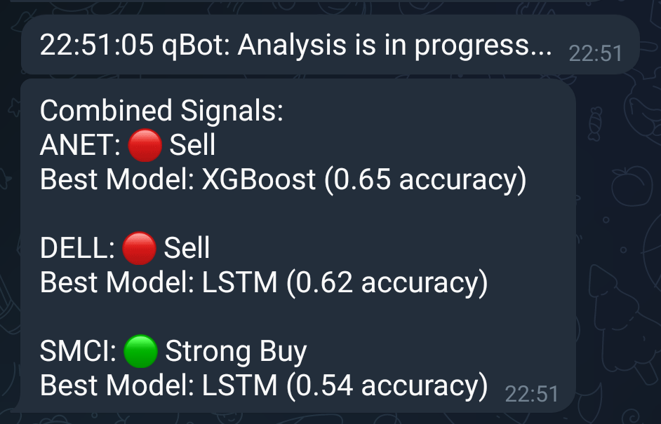
Excellent, so we have a working bot, with analysis, back-testing and predictions, but, the accuracy is quite low, so this will be my next item to work on (or rather AI to work on).

pxng0lin.