Welcome to another blog on Machine Learning! Today we are going to have a look at the Decision Tree Regression.

Intuition

There is a term called CART which stand for classification and regression tree. In this blog we’ll talk mostly about regression tree cause this is more complex than a classification tree.

Let’s have a look in this scatterplot. In the plot we have two independent variables x1 and x2. And what we are predicting is a 3rd dependent variable which is Y (a 3rd dimension)

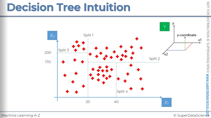
You see there are many splits in the plot. When we apply the regression tree, it splits the plot into many parts and the splits are decided by the regression tree model. The splits, the line is called leaf. These splits actually increases the amount of information to our plot. The algorithm knows when to stop when there’s a certain minimum value for the info that needs to be added. Another point is that the algorithm will stop creating leaves if a leaf ends up with less than 5% of the data. The algorithm is able to handle this and it finds the optimum splits of our data set into these leaves, the final leaves are called the terminal leaves.

What is actually populating into those boxes?

We will explore how to predict the value of Y for a new observation added to our scatterplot. Let's say x1, x2 = (30, 100), so the observation falls into the box between 20 and 40. What we are going to do is pretty straightforward. We simply take the average of Y for all the points in our terminal leaves. This average will be the value assigned to any new point that falls in the terminal leaf.

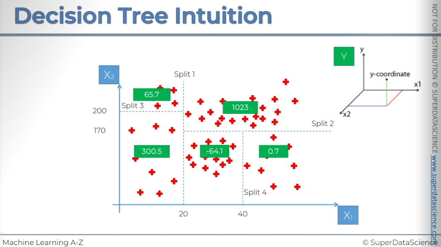
These are the averages. the prediction model will predict a value of -64.1 for y. That’s how we can predict more accurately the value/assign the value of y to a new coming element. This is the whole point of regression.

Python Steps

Resources

1. Decision regression tree colab file: https://colab.research.google.com/drive/14z4MBI_rjrF4i2p3Ofo1OT03Zd5WDuyy

2. Data sheet: https://drive.google.com/file/d/1rCIbvYTYYsKjP2a6XbwsW7eYKDHm3asy/view

3. Data preprocessing template: https://colab.research.google.com/drive/17Rhvn-G597KS3p-Iztorermis__Mibcz

The first step, delete all the code cells and import the data preprocessing tools and change the data sheet name.

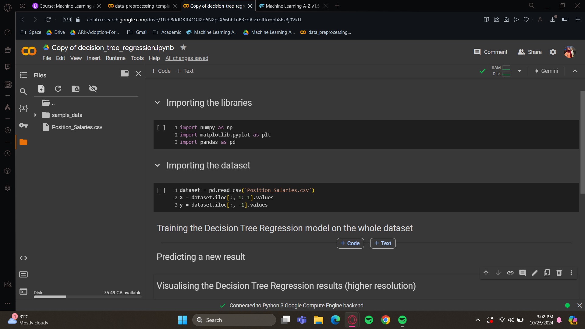
Training the Decision Tree Regression model on the whole dataset

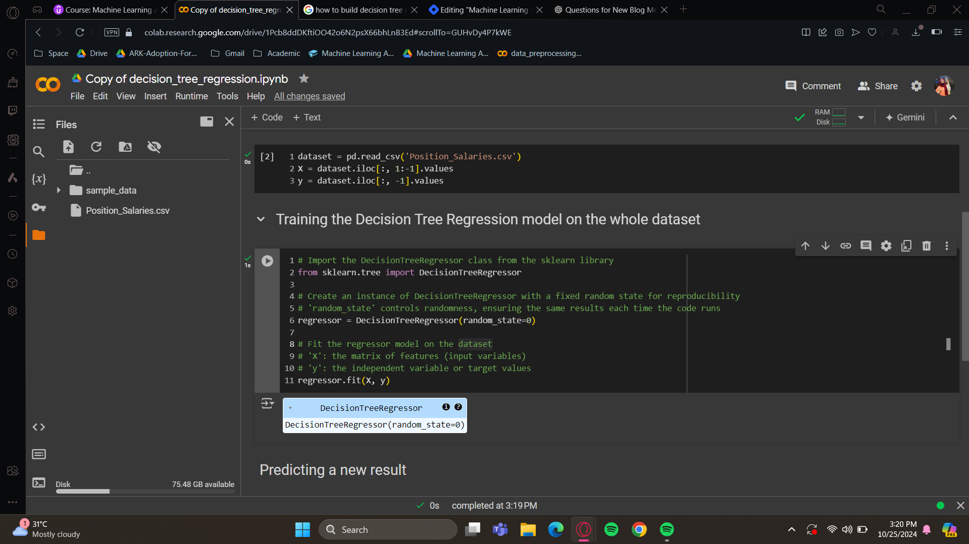
For training purposes, the random state parameter helps us get the same result each time. There are some random factors involved when building and training your DecisionTreeRegressor. If we don't fix the seed, we'll get slightly different results. It's better to have consistent results so everyone can be on the same page. So, we'll set the random_state parameter to zero. This fixes the seed with the zero value for the random_state parameter.

Predicting a new result

To make the prediction, since no feature scaling is needed for decision tree regression, we just call the predict method on our regressor. We input the observation 6.5, formatted in a 2D array, to get the corresponding salary.

The predicted salary from the decision tree regression model for our case study is $150,000. This prediction is lower than the requested salary, which isn't ideal. The decision tree regression model isn't the best choice for a single feature dataset; it's better for datasets with many features. However, the code can easily be adapted for other datasets. I'll still show you the visualization results in 2D to demonstrate the regression curve, even though it's not well-suited for this model.

Visualising the Decision Tree Regression results (higher resolution)

(copied the code from polynomial) We'll start with this code, and your task is to make the necessary changes for it to work with the Decision Tree Regression model. If you succeeded with the SVR model, this will be easy since no feature scaling is needed, so you won't need to use the transform or inverse transform methods.

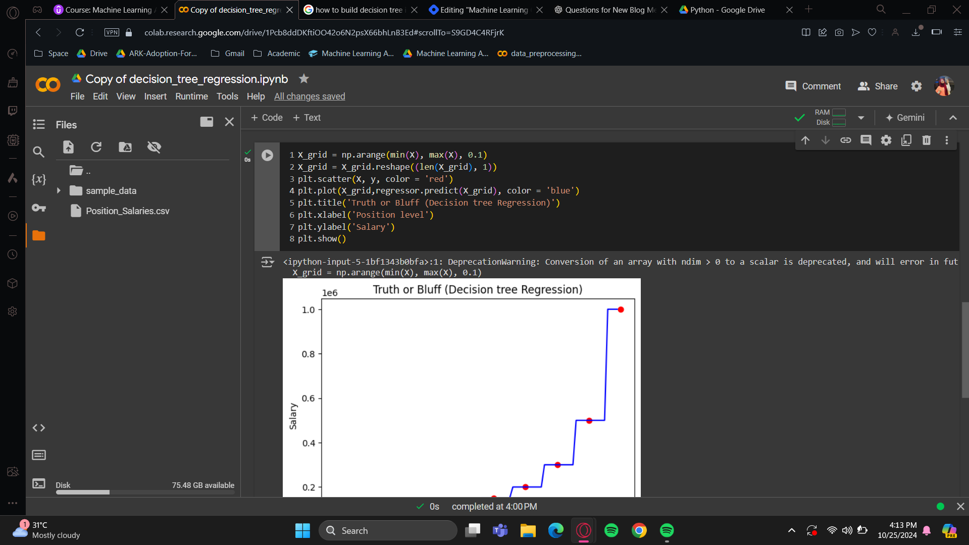
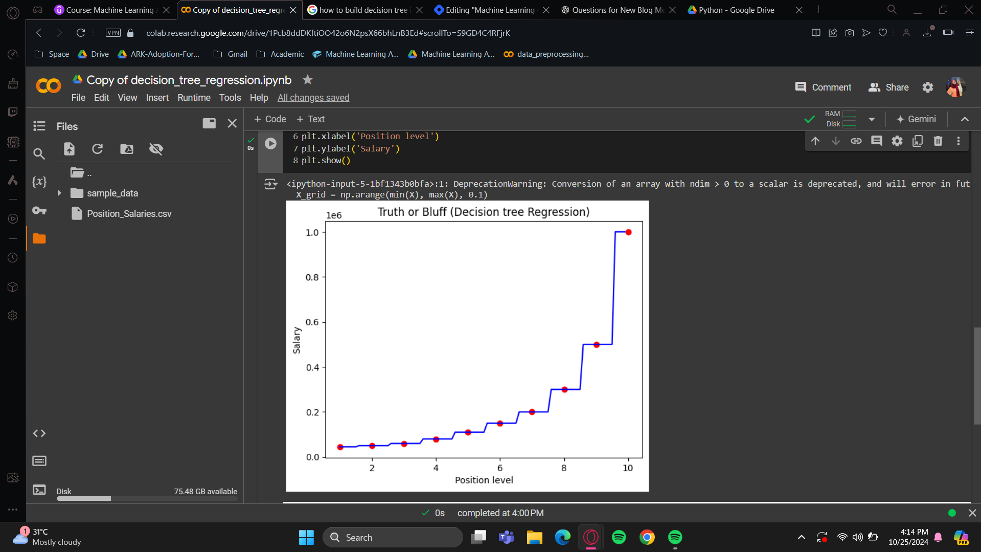
What this Decision Tree Regression model did was take the actual salaries for each position level and predict the same salary for all levels from position level minus 0.5 to position level plus 0.5. It predicted the salary to be the same as the level in the middle. This approach is understandable and intuitive because as you know, decision trees work by splitting data through successive nodes. In the end, you get different feature ranges where the prediction remains the same. Here, all the predicted salaries within this range of position levels are the same, that’s why we get a stair-step curve up to the last position level. This is not continuous; it's actually a series of vertical bars. So, the regression curve jumps from one position level to the next with each step. It's not very pretty or relevant in 2D, but I still recommend trying the Decision Tree Regression model for higher-dimensional datasets because it can perform well.

Okay that was it. In the next blog we’ll learn about Forest Regression Model.

Enjoy Machine Learning!