Finding the Best-Fit Line in Linear Regression – Manual Minimization vs. Gradient Descent
 Deepak Kumar Mohanty
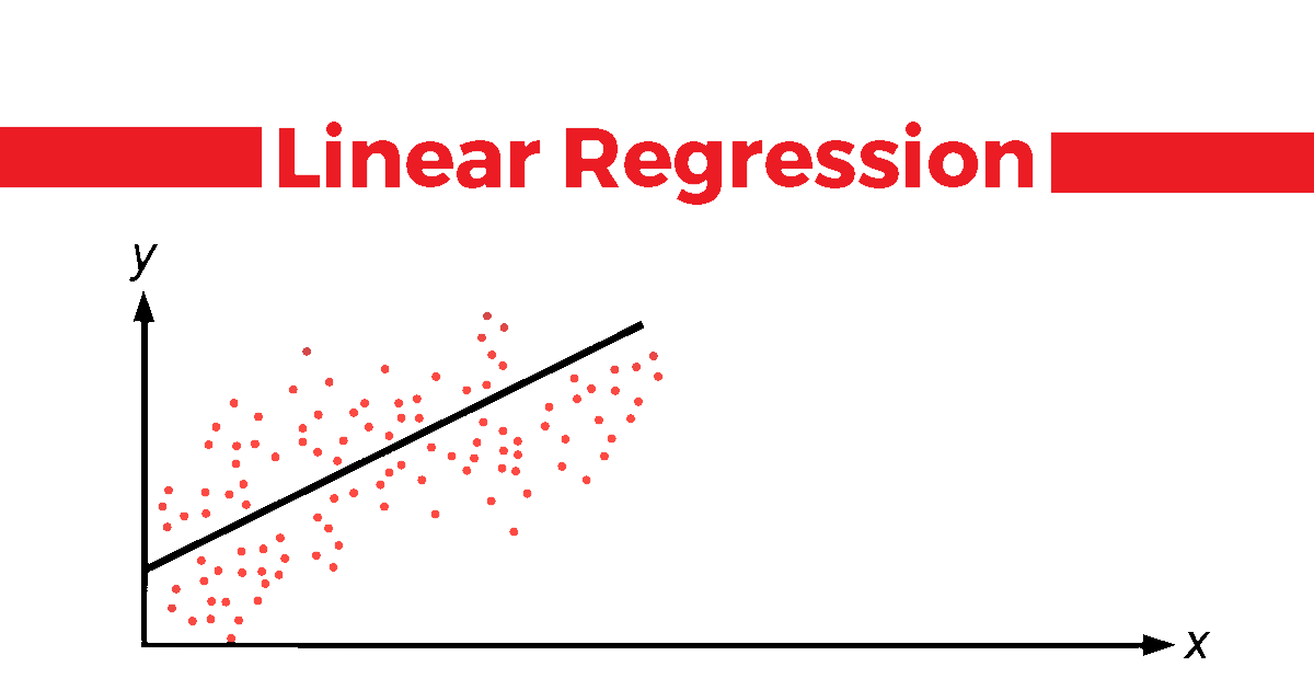
When working with linear regression, the goal is to identify the best-fit line that captures the relationship between your input (independent) variable x and output (dependent) variable y. This line, represented by the equation:
$$h_{\theta}(x) = \theta_0 + \theta_1 x \quad \text{or} \quad \hat{y} = m_i \cdot x + c_i$$
is our model's predicted value of y for a given x. Here, θ₀(theta_0) is the intercept (c) , and θ₁(theta_1) is the slope (m) of the line, which tells us how steeply the line rises or falls. But how do we find these values of θ₀ and θ₁ to fit the line most accurately?
In this article, we’ll compare two key methods for finding the best-fit line: Manual Minimization of the Cost Function and Gradient Descent Optimization.
Approach 1: Manual Minimization of the Cost Function
In manual minimization, the strategy is to test different values for θ₀ and θ₁ to minimize the cost function, also known as Mean Squared Error (MSE). This cost function helps us quantify how close our predictions are to the actual data points:
where:
m is the number of data points,
hθ(x⁽ⁱ⁾) is the predicted y-value for a given x-value,
y⁽ⁱ⁾ is the observed y-value.
The goal is to find values of θ₀ and θ₁ that minimize this cost function. Here’s how it works step by step:
Step-by-Step Process:
Define the Cost Function: Start by defining how far off each predicted value is from the actual values.
Test Different Values: Choose initial values for θ₀ and θ₁ (for example, start with zeros). Calculate predictions, put them into the cost function, and check the error.
Iterate with New Values: Adjust θ₀ and θ₁, calculate the cost again, and look for the smallest cost. Keep testing different combinations until you find the values with the lowest cost.
Limitations of Manual Minimization
While this method is intuitive and easy to understand, it has limitations:
Time-Consuming: Testing values one by one can take a long time, especially with large datasets.
Imprecise: It’s challenging to reach high precision since the manual trial-and-error approach is inherently limited.
Approach 2: Gradient Descent Optimization
Gradient Descent is a systematic and efficient approach to minimize the cost function without relying on trial and error. Rather than randomly guessing values for θ₀ and θ₁, Gradient Descent uses the slope of the cost function to guide adjustments.
Step-by-Step Process:
Initialize θ₀ and θ₁**:** Start with initial values (again, typically zeros or any other starting guesses).
Calculate the Cost Function: Like in manual minimization, we define our cost function as the sum of squared errors.
Compute the Gradient (Slope of the Cost Function): Calculate partial derivatives of the cost function with respect to θ₀ and θ₁. These derivatives (gradients) tell us the direction to adjust our parameters to reduce the cost:
the above can also be written as :
- Update θ₀ and θ₁ : Use the gradients to adjust θ₀ and θ₁ with each step, guided by the learning rate η(eta) , a small positive value (e.g., 0.01 or 0.001). This prevents overshooting or slowing down the process:
- Repeat Until Convergence: Repeat steps 3 and 4, recalculating gradients and adjusting parameters until the cost function decreases to a minimum or until the updates become very small.
Why Gradient Descent Works
Gradient Descent efficiently finds the best-fit line for large datasets, as it uses the cost function's slope to direct the adjustments, enabling fast convergence toward the minimum error.
Comparing Manual Minimization and Gradient Descent
| Feature | Manual Minimization | Gradient Descent |
| Speed | Slow; manually tries values | Fast; automates parameter adjustments |
| Ease of Use | Time-consuming, impractical for large data | Efficient and widely used in ML |
| Precision | Often imprecise | Highly precise with minimized cost |
| Automation | Manual trial-and-error | Systematic and efficient |
Summary: Which Approach is Better?
For real-world applications, Gradient Descent is the preferred method. It’s faster, automated, and more accurate than manually testing values. The method's iterative adjustments based on the cost function's slope allow it to find the best-fit line with minimal error, making it a cornerstone in machine learning.
Explore More Insights
If you found this article helpful, you might also enjoy these previous posts:
Subscribe to my newsletter
Read articles from Deepak Kumar Mohanty directly inside your inbox. Subscribe to the newsletter, and don't miss out.
Written by

Deepak Kumar Mohanty
Deepak Kumar Mohanty
Hi there! I'm Deepak Mohanty, a BCA graduate from Bhadrak Autonomous College, affiliated with Fakir Mohan University in Balasore, Odisha, India. Currently, I'm diving deep into the world of Data Science. I'm passionate about understanding the various techniques, algorithms, and applications of data science. My goal is to build a solid foundation in this field and share my learning journey through my blog. I'm eager to explore how data science is used in different industries and contribute to solving real-world problems with data.