ML Classification: Logistic Regression
 Fatima Jannet

Welcome to part 3!
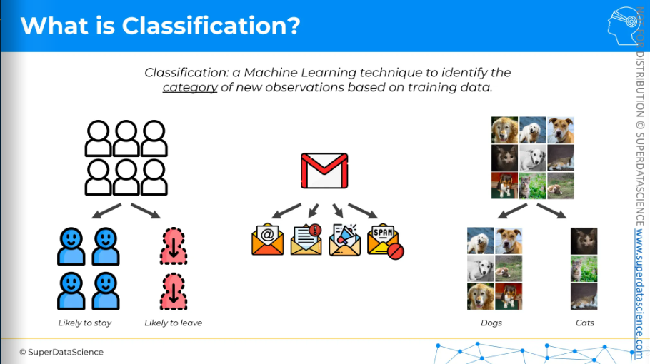
In regression we used to predict a continuous number. But in classification, we will predict a categorical value. Wide variety of classification models are used in machine, marketing, business medicine; such as: Logistic regression, SVM and non-linear ones like K-NN, Kernel SVM and random forest.
The fields are, for example: business where you would like to predict which one are likely to stay and who are gonna leave (churn modeling, very important), email classification, imagine recognition and so on!
Int his classification part, I will cover
Logistic Regression
K-Nearest Neighbors (K-NN)
Support Vector Machine (SVM)
Kernel SVM
Naive Bayes
Decision Tree Classification
Random Forest Classification
This blog will cover Logistic regression. Enjoy!
Logistic regression intuition
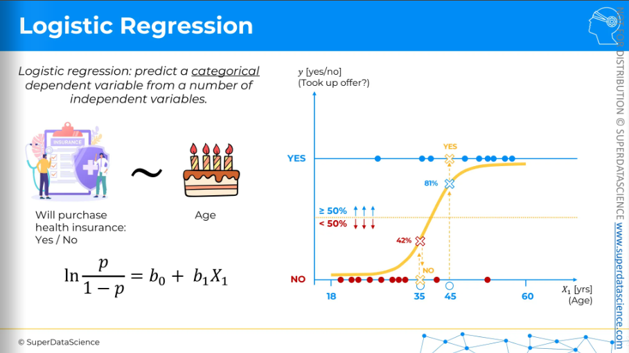
The key difference from linear regression is that we're predicting a categorical variable, not a continuous one. For instance, in an insurance company, you might predict if someone will buy health insurance—yes or no. This prediction is based on an independent variable like age. On the x-axis, we have age, and on the y-axis, we have yes or no, indicating if they accepted the offer.
(sigmoid curve). We want a yes/no answer that’s why we have set a middle line where > 50% means NO(Binary 0) and >50% means YES.
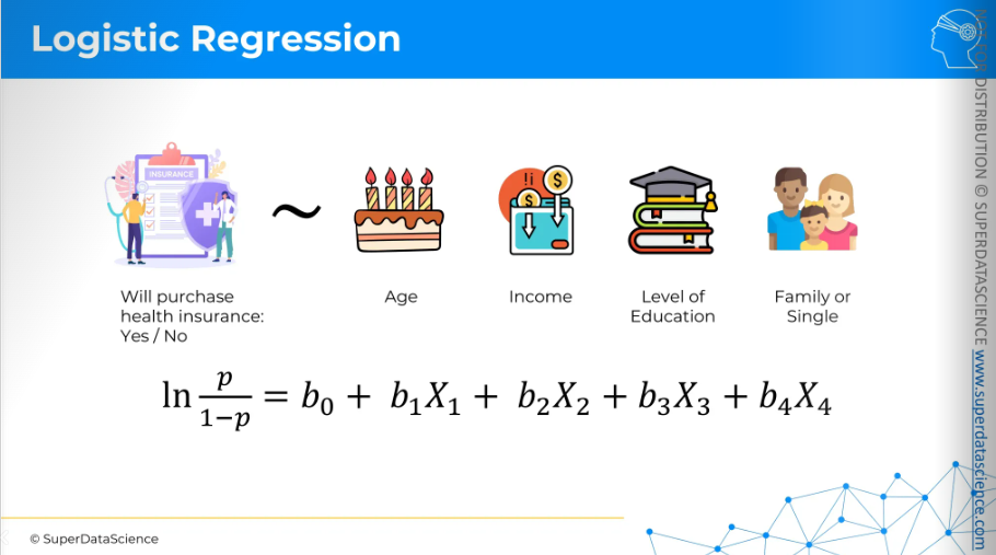
And just like linear regression, you can have multiple independent variables, such as age, income, education level, and family size. Other variables can be added depending on the use case. That's logistic regression in a nutshell.
Maximum Likelihood
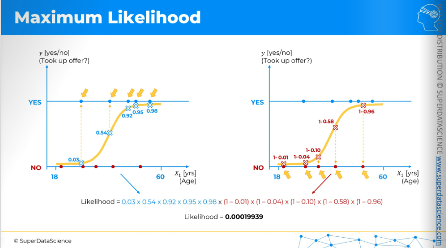
These two plots are the same but to avoid cluttering, I have plotted yes/no into two plots. On the right side, they are the probability of saying YES (taking up the offer). So the probability of them saying NO are 1-that value.
So, 1 - probability of saying YES = probability of saying NO
Likelihood is calculated by simply multiplying all these numbers. On the blue side, we multiply these numbers, and on the red side, we multiply those numbers. This gives us our likelihood value. Then, we find the best-fitting curve.
The way to find the best fit is to look for all possible sorts of curves. The process is more sophisticated, but in a nutshell, we compare the likelihoods of different curves.
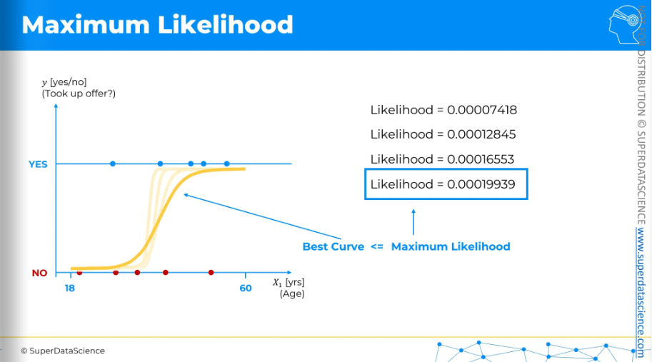
Let's say our logistic regression modeling process started with this curve and calculated the likelihood to be a certain value. Then it moved to the next curve and calculated the likelihood for that one. It continued to the next curve, calculating the likelihood each time. Through this iterative process, it found the curve with the highest likelihood. This means it is the best-fitting curve. So that’s how maximum likelihood is calculated.
Logistic regression in Python steps
This time, we won't predict a continuous numerical value, like in part two with regression. Instead, we will predict a category.
Resources:
Data sheet: https://drive.google.com/file/d/1wzpfJYPBvP0unhxZDLHh5HgRd6I3M43C/view (download)
Colab file: https://colab.research.google.com/drive/1-Slk6y5-E3eUnmM4vjtoRrGMoIKvD0hU (make a copy of it)
Data pre processing template: https://colab.research.google.com/drive/17Rhvn-G597KS3p-Iztorermis__Mibcz
Let’s imagine you are a data scientist of your favorite car company. Your company has release a brand new SUV and the manager has asked you (the most intelligent data scientist) to predict which of their previous customer will likely to buy the brand new SUV. Your mission is to predict which of your previous customer will buy a brand new SUV.
For this purpose you’ll need data to train on your ML model. That’s exactly the data your manager has provided you. Each of the column represents a customer’s age, salary and the dependent variable purchase history(binary). Your model will be trained on this data and for the new customer’s we’ll predict if they will buy a new model or not.
Importing data and feature scaling
Import the libraries and add datasheet
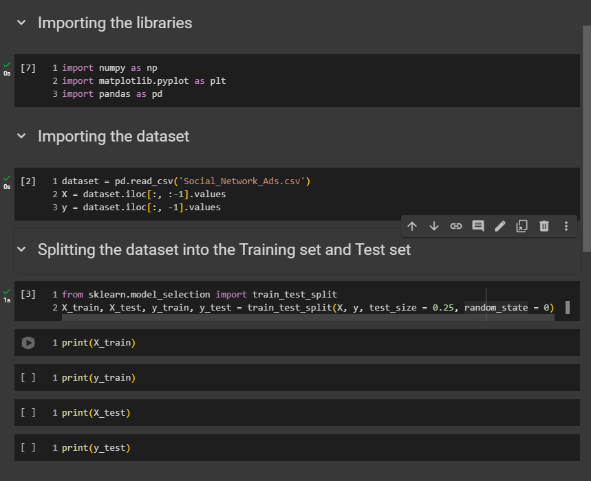
I want to remind you that it is absolutely necessary to do this after splitting the dataset into the training set and test set to avoid information leakage from the test set. Also, we don’t apply feature scaling to Y.

Run all the codes so far.
Training the Logistic Regression model on the Training set
Resource:
- https://scikit-learn.org/stable/ - this is the link of scikit learn homer page. From here you ca n got to APIs. Here you will find every possible things you can do with scikit learn.

The random_state=0 parameter is used to ensure reproducibility of results by controlling the randomness involved.
Predicting a new result
Now we will predict whether a new customer in the test set will make a purchase. This customer is the first one listed, who is 30 years old and earns an estimated salary of $87,000.
If you look at your test set X_test, before scaling, the first one is the exact customer you need to input into your predict method to determine the purchase decision. To check if he has purchased any car before, go to y_test because y_test contains the purchase history. In our case, he didn’t buy any car previously from our company.

the predict method expects from its input a two dimensional array.
input the two values
of these two features, the age and the salary.
Predict methods can only be used on observations where features have the same scale as the training data. So, we need to use the transform method to ensure the predict method has the correct format and scale.
We need to take our SC object, the feature scaling object, which was used to apply scaling on both the training set features
X_trainand the test set featuresX_test.
Okay, so we got zero. Our model did amazing performance to predict.
Predicting the Test set results
Now we will predict some real purchase decisions.
Resource:
- Multiple linear regression: https://colab.research.google.com/drive/1Lp16gstLKT6DfhTPNsbwdG3BgEjWDZIO
From here, you will find the “predicting the test result” template. We have implemented it many times.( We have all the same names. Using templates are honestly efficient)
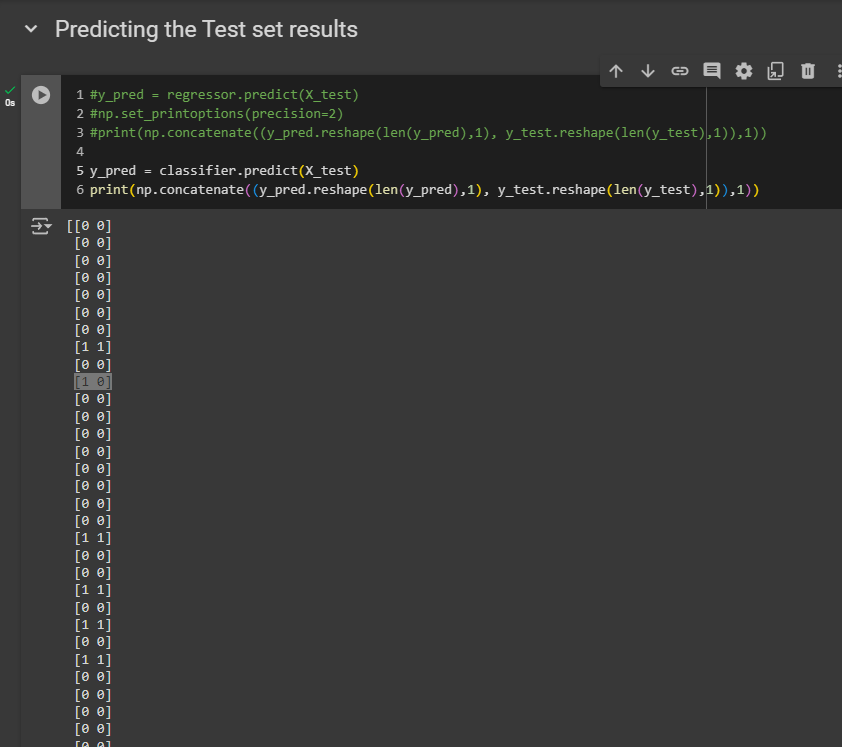
Well, in this time - we are dealing with either 0 or, 1 so we don’t need to precise anything how how many digits we want after the digit. That’s why I have removed the precision part.
We got two vectors. The left column shows the predicted decisions and the 2nd column is the real purchase history. By comparing the predicted one with the real one, you can check how well your model (based on X_test) has predicted results. You will find some errors but still the accuracy is really good of this model.
Now, we will make an accuracy.
Making the Confusion Matrix
Looked here to see what I need to include in my confusion matrix.
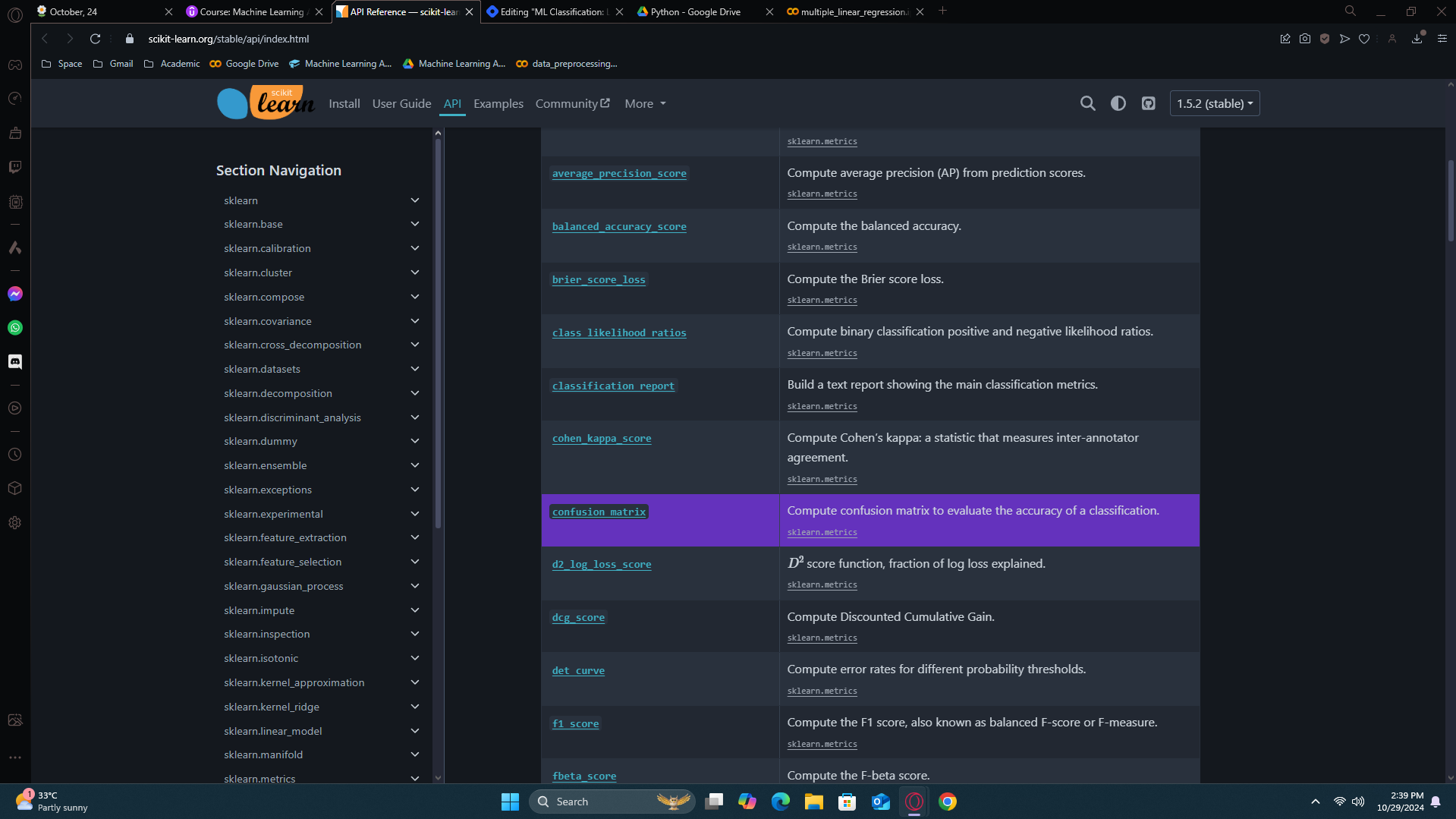
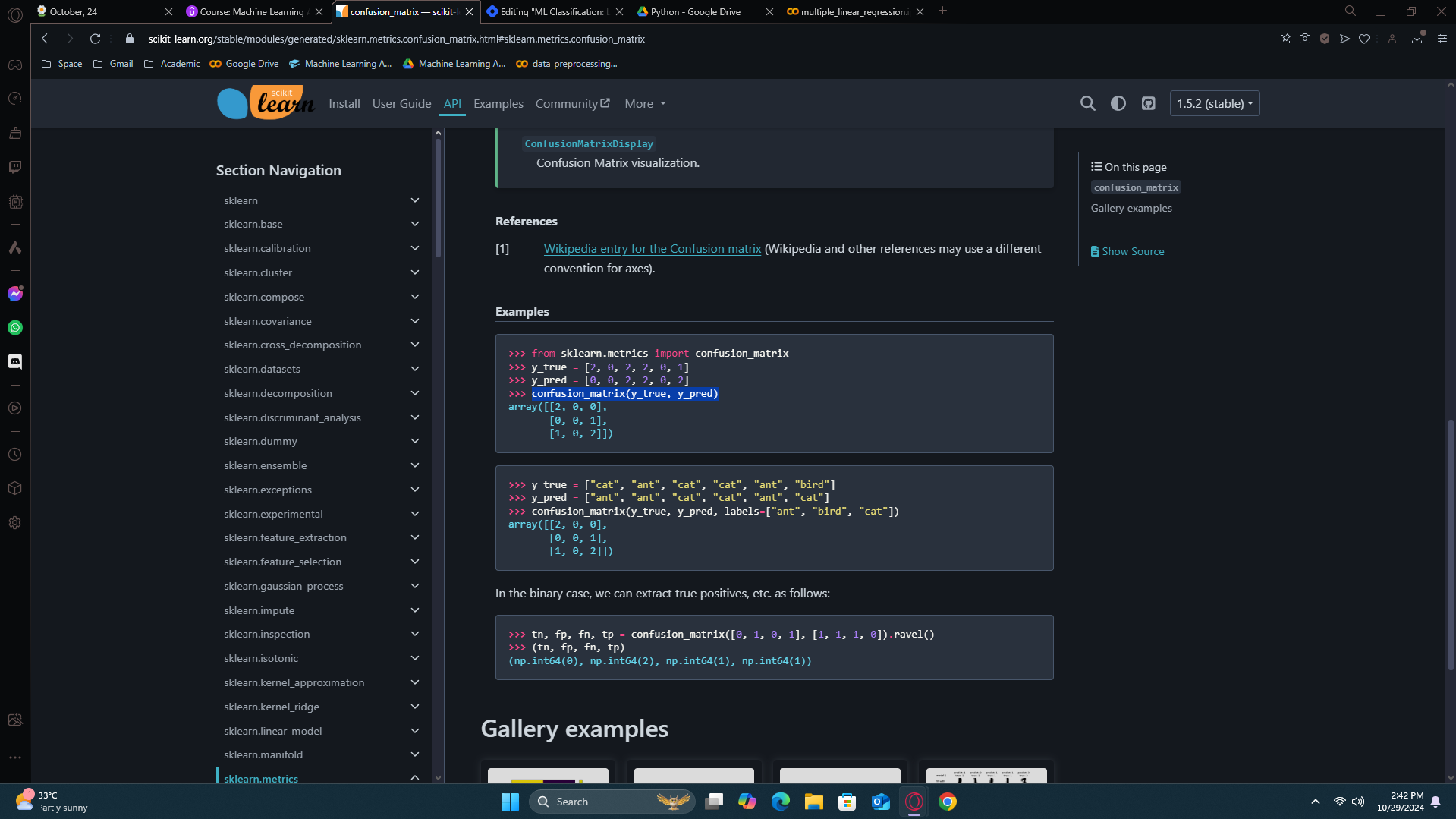
Note: I'm not doing this because I'm lazy. I'm doing this to help you become independent and learn how to find things on your own.
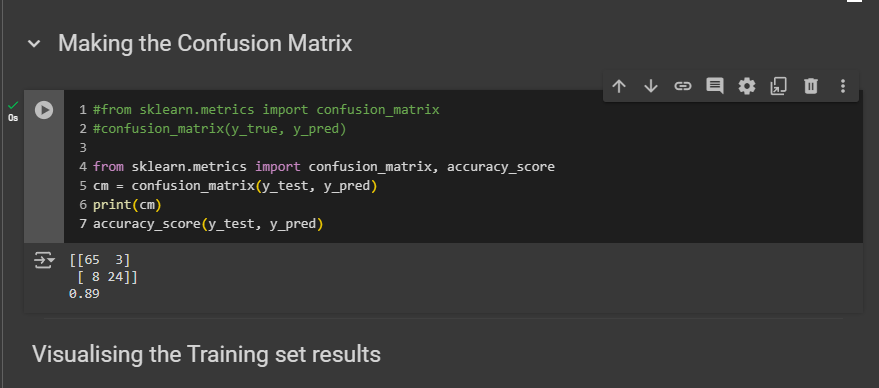
65 correct predictions of class 0, meaning those who didn't buy the SUV.
24 correct predictions of class 1, meaning correct predictions of customers who bought the SUV.
Three incorrect predictions of class 1, meaning three customers who actually bought the SUV were predicted not to.
Eight incorrect predictions of class 0, meaning eight customers who didn't buy the SUV were predicted to buy it.
Finally, we achieved 0.89, meaning we had 89% correct predictions in the test set. Remember, there are 100 observations in the test set, so we indeed had 89 correct predictions. Specifically, 65 plus 24 equals 89. Alright?
Visualising the Training set results
we're going to visualize on a 2D plot the prediction curve and regions of the logistic regression model. The X axis shows the first feature (age), and the Y axis shows the second feature (estimated salary).
Note: You will probably never use this visualization because it requires only two features, and in your future tasks, you'll usually have more than two features. This code is quite advanced, and not only is it advanced, but you'll likely never need to use it again in your career. If you want to understand it, that's fine, but if you can't, that's okay too. It's perfectly fine if we don't go into detail on this code because it's just for training purposes. It's meant to show you the differences between linear and non-linear classifiers, and you probably won't use it again in your future machine learning projects.
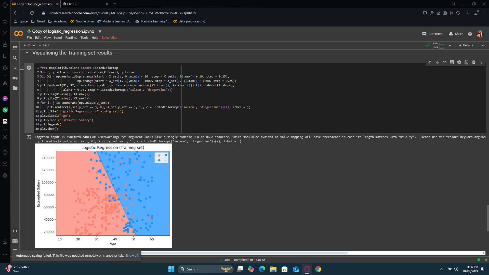
The blue points represent the customers who bought the SUV, and the red points represent the customers who didn't buy the SUV, shown as zero here. There are incorrect prediction too, as you can see, which fell into the wrong region.
Visualising the Test set results
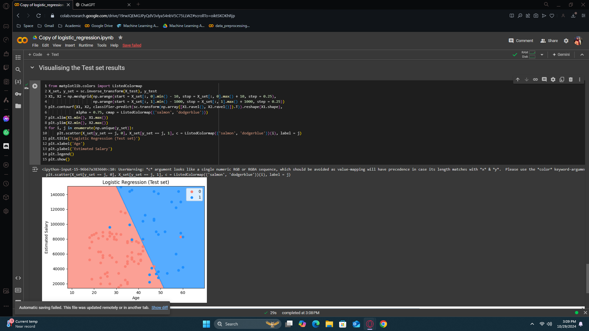
Our prediction model performed well in predicting the results. However, we want our model to have fewer errors. How do we achieve that? We need a prediction boundary or a curve that will take a different path and capture all the errors along the way.
However, that's for another day. We'll learn how to do it later.
Subscribe to my newsletter
Read articles from Fatima Jannet directly inside your inbox. Subscribe to the newsletter, and don't miss out.
Written by
