Hello and welcome back to the ML blogs. Today we will learn about the K nearest neighbor. Let’s get started!

Intuition

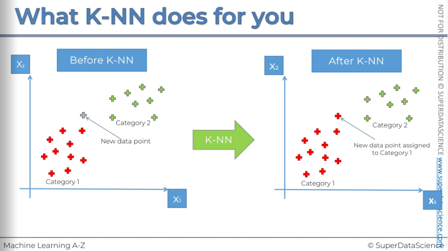
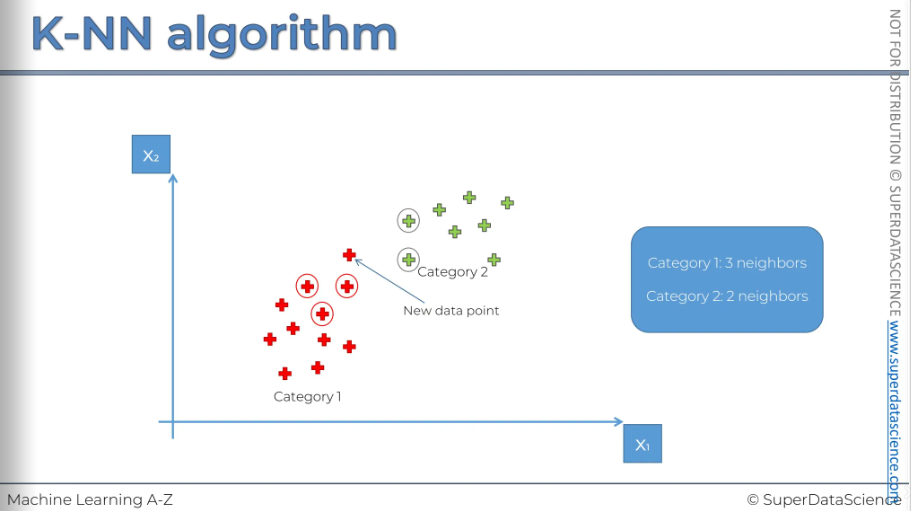
Let’s say you have a plot where you have two types of category, red data and green data. Now, if a new data point appears where should we place it? Well, K-NN assists us in these type of problems. This algorithm figures out where to put the data. For example, in this case, it has put the data in the red region.

How does it works?

There is a step-by-step process which is, very simple.

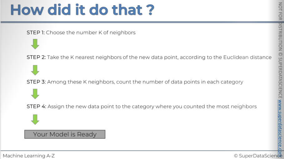
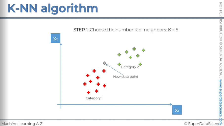
So here we've the new data point that has been added to our scatterplot. Ho do we find the nearest neighbors of this new datapoint?

Start with step 1: K = 5 (commonly used).

Well, let’s have a look at the Euclidean Distance. If P1 is a point and P2 is another point than the distance between them is this formula. This is the geometric distance. So basically on a scatterplot a two dimensional kind of polygon just draw the lines and see what is closer.

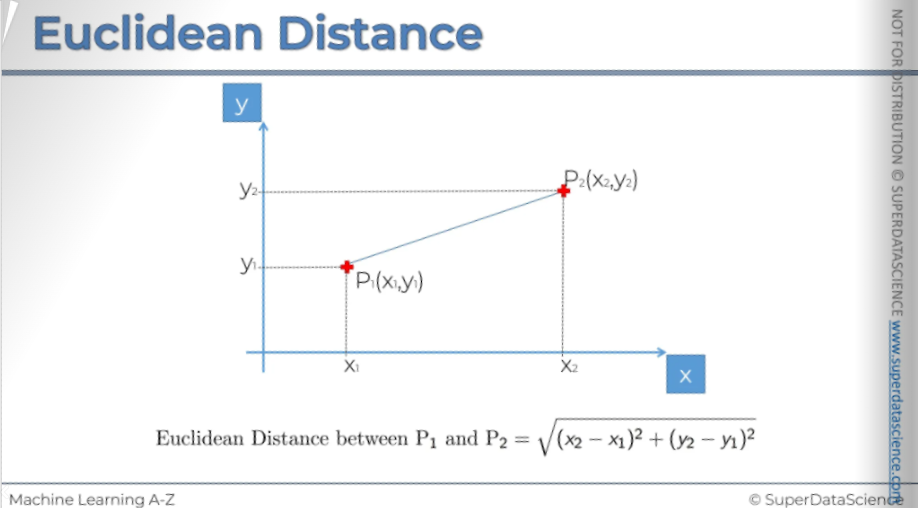
So here, on the scatterplot, we just look at them and we check the distance between them to see which one in the nearest.

After that, step 3: among these Cockayne neighbors count the number of data points in each category. In category 1 we have 3 neighbors and in category 2 we have 2 neighbors.

Step 4: mare assigned the new data point to the category where you counted the most neighbors. Which means we need to assign it into the red category.

As simple as that. We have classified the new data point, This is a very straightforward process.

Python Steps

Resources:

1. Colab file of K-NN: https://colab.research.google.com/drive/14Jn7Yx3Fbonk1sEqxZzT0txIEuqyR160 (make a copy of it)

2. Data sheet (contains 400 observations): https://drive.google.com/file/d/1zFz5TYlB94KgRbT15FANANPhkZfdK3t2/view (download it and add to the copy of K-NN)

Now if you would look at Logistic regression, you will find all the codes are similar except the last ones. For K-NN, we will just reimplement our codes. \

Training the K-NN model on the Training set

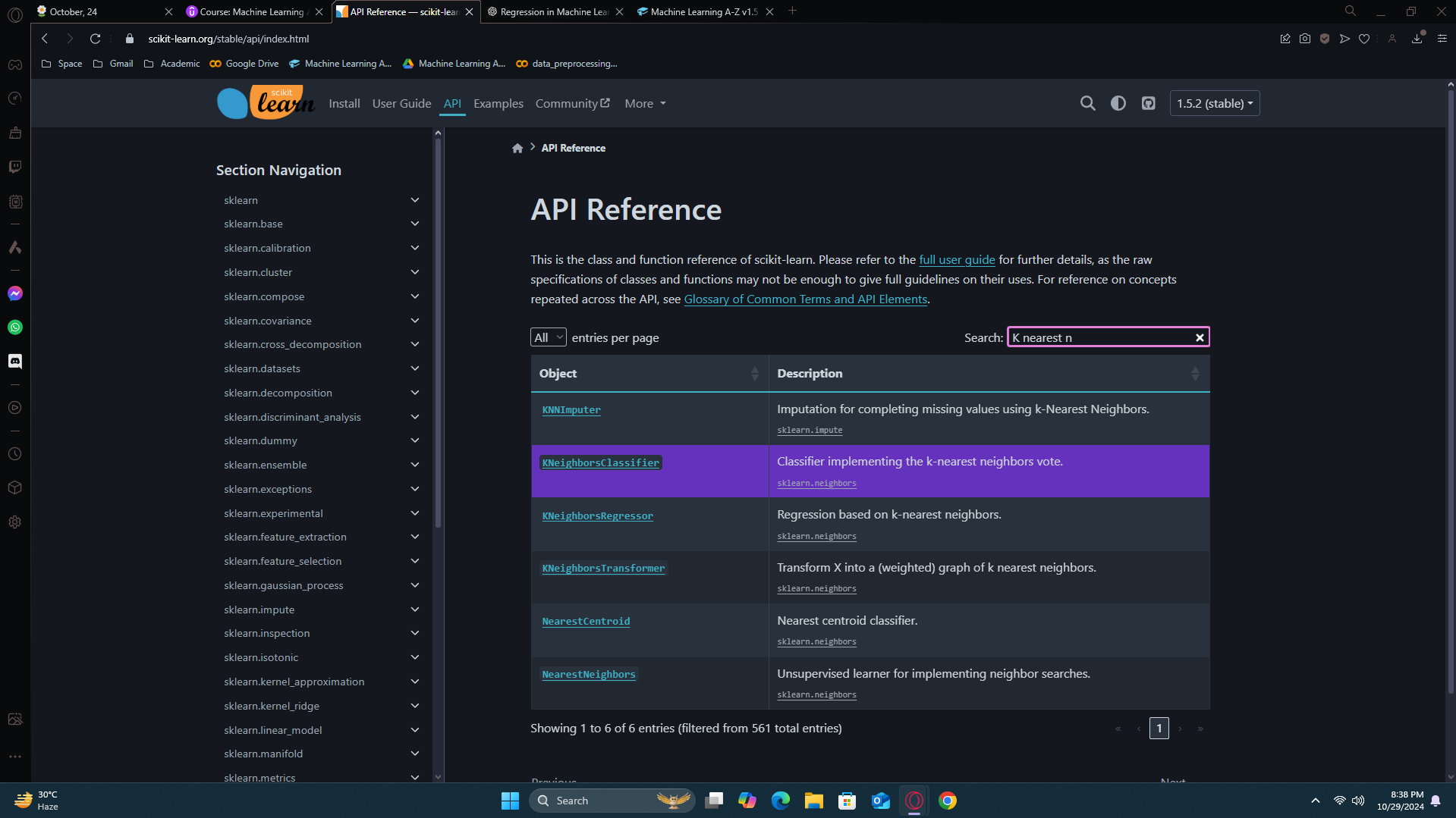
Go to this section cause rest are similar. Try to do it on your own from scikit learn website.

[API contains all the modules, classes and functions of scikit learn]

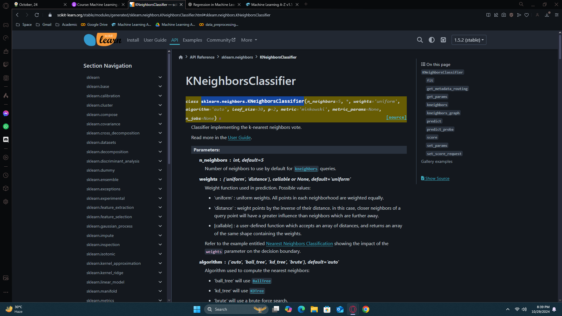
[the class and the params. While creating an object, you will find if you need to add any params and if yes, what type of params]

And here it is. I found what i need to put based on the website.

You can run all now. Everything is same as logistic here.

Making the Confusion Matrix

Okay, i can see the errors are really less here, 4+3, 7 errors in total. And the accuracy is 93% which is really really great.

Visualizing

While running, we might see that visualizing is taking a lot of time. Well that’s because K-NN is actually very compute intensive, there are a lot of computation on running K-NN.

Training set results

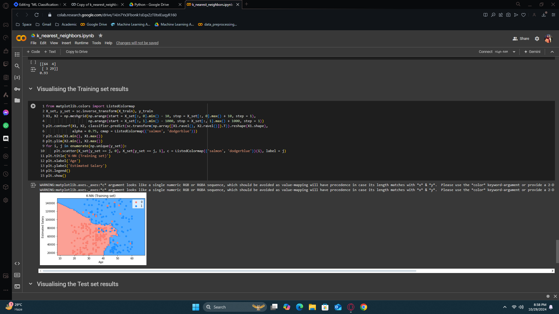
Remember, with the logistic regression classifier, the prediction boundary was a straight line. Cause, the logistic regression model is a linear classifier. Always remember, for linear classifiers, the prediction boundary is a straight line. In three dimensions, it's a plane, and in N dimensions, it's a hyperplane. And so here we had a straight line, which therefore resulted in having a lot of incorrect predictions.

In logistic regression, we were hoping for a curve which will catch the errors along in it’s way - so, here we got our K-NN to do that. We didn’t get a smooth curve but we got something that catches the errors.

Test set results

On the test results, we again got an excellent results. the K-NN prediction curve or prediction boundary or even decision boundary catches all the right customers.

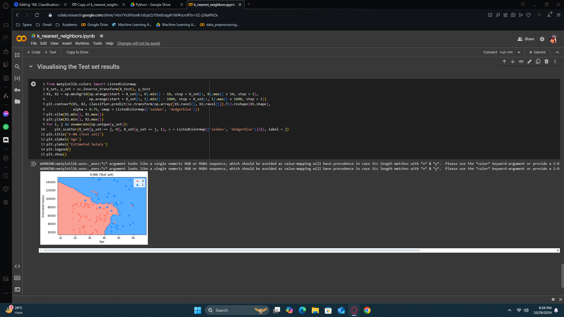
This is already much better. The accuracy level went upto 4%.

Can we do even more better than this? Let’s find out on the next blog!

Enjoy Machine Learning!