Optimal Storage for Trading Factors Calculated at Mid to High Frequencies
 DolphinDB
Maintaining a large number of factors is a common challenge in quantitative analysis. In many cases, the volume factor data can far exceed that of high-frequency market data. For example, calculating factor data for a year across 5,000 securities can yield substantial volumes: 10-minute intervals would generate 2.3TB yearly, 1-minute intervals 23TB yearly, and 3-second intervals 460TB yearly. This massive amount of data requires thoughtful storage solution planning.
This tutorial compares different DolphinDB storage solutions for factors calculated from high-frequency data using real-life scenarios to provide recommendations for efficient storage.
1.1. The Challenges
The high frequency of data generation coupled with the massive number of factors results in huge data volumes, often reaching the terabyte level. The storage solution must effectively address the following challenges:
- Massive Data Volume
Factor calculations involve four aspects: securities, factors, frequency, and time. For example, assuming:
There are approximately 5,000 securities listed in the market.
Most teams use around 1,000 factors, though some may have as many as 10,000 factors.
Data is generated at varying time frequencies, ranging from 3-second to 10-minute intervals.
That is to say, assuming 4 hours of daily trading, a single factor for a single security generates 24 to 4,800 ticks per day.
The volume of factor data varies significantly depending on the storage format. In wide format, where each factor has a separate column, the data volume is as follows:
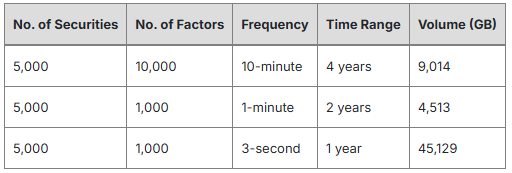
In narrow format, where data is stored with columns for timestamps, security IDs, factor names, and values, respectively, the data volume is as follows:
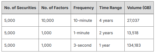
Note: For details of how data is stored in wide/narrow format, see section 3.1 Designing Storage Solutions.
With such massive data, ensuring efficient data writing and compression rates is critical. Inefficient practices can lead to hours of data writing without parallel I/O of disks.
- Changes in the factors
The factor library undergoes frequent changes, including adding new factors, modifying definitions, or incorporating new securities. Given the terabyte-scale data, these additions, modifications, or removals must complete within seconds to ensure efficient quantitative research.
When designing factor storage solution, it’s important to ensure that none of these operations becomes a notable performance bottleneck. Otherwise, as data volume rises, the overall efficiency will significantly decrease.
2. Alignment of factors
To facilitate quantitative analysis, it is common practice to align the factors of a security in the output. In situations where we query multiple factors of a single security (e.g., selecting 1,000 factors from a pool of 10,000 factors for 1 out of 5,000 total securities), queries must be fast and precise to minimize inefficient I/O, and output the factor values in the desired format, typically in a panel structure.
1.2. The Requirements
To address the aforementioned challenges, an ideal storage solution for high-frequency factors should meet the following criteria:
High writing efficiency
Smooth factor library maintenance, including additions, modifications, and removals of factors.
Quick and flexible queries with factors aligned in the results, serving as an ideal basis for further analyses.
2. Storage Capabilities of DolphinDB

2.1. Database Partitioning
Factor data can be composite partitioned based on two commonly used query conditions, date + factor name, or date + security name. Operations on different partitions can be performed concurrently in DolphinDB.
2.2. In-Partition Sorting
The DolphinDB TSDB storage engine allows users to specify “sort key“ that acts as an index for the data blocks within each partition. This enables the storage engine to quickly locate data for random queries. For example, within the “2022.02 — factor1” partition, data is sorted based on the “SecurityID“ column (i.e., the sort key); and for data sharing the same SecurityID, further sorting is applied based on the time values in the time column “TradeTime“ (see image below).
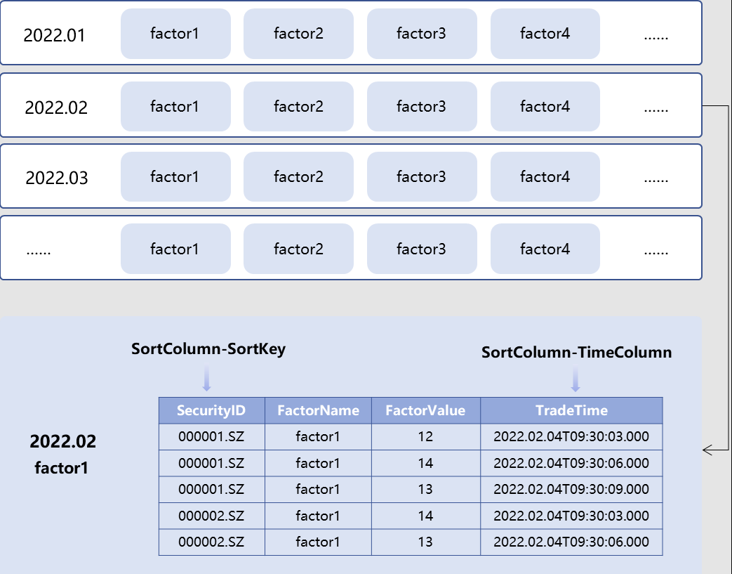
These capabilities of DolphinDB can be leveraged to provide a flexible storage solution for high-frequency factors.
In the following sections, we will compare the performance of two storage solutions based on the scenario where data for 10,000 factors at 10-minute intervals. Our goal is to evaluate the write, query, and maintenance operations of each storage solution and determine the optimal one for storing high frequency factors in DolphinDB.
3. Storage Solutions: 10-min Frequency Data for 10,000 Factors
3.1. Designing Storage Solutions
There are two main formats for storing factor data — narrow and wide.
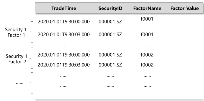
As shown in the image below, the narrow format table has four columns, holding timestamps, security IDs, factor names and factor values. Using the pivot function/keyword, narrow data can be transformed into the panel format, where each row represents a unique combination of a timestamp and a security ID, and each factor is presented in a separate column. This allows calculations on both dimensions with optimized performance.
The wide format has a separate column for each factor, as shown in the image below. This format can be used directly in quantitative analysis as it aligns multiple factors of each security along timestamps.
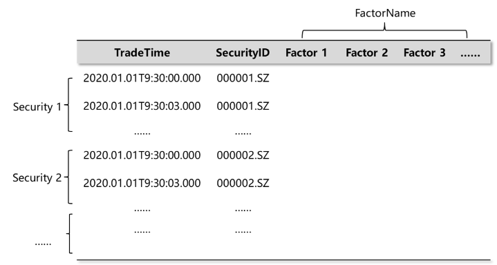
DolphinDB supports both narrow and wide formats for data storage. We designed the following two solutions to store data for 10,000 factors generated at 10-minute intervals.
Solution 1: Narrow Format Storage
Partition data by month (using TradeTime column) and factor name (FactorName)
Within each partition, sort data by security ID (SecurityID) and trade time (TradeTime)
The key advantages are: (1) Keeps each partition at an appropriate size; (2) When executing queries, the system can pinpoint the relevant partitions by filtering on month and factor name (i.e., partition pruning). It can then efficiently retrieve the target records within each partition via SecurityID.
Solution 2: wide format storage
Partition data by month (TradeTime) and security (SecurityID)
Within each partition, sort data by security ID (SecurityID) and trade time (TradeTime)
Partition pruning is carried out by filtering on month and security ID. The queried factors are retrieved from the corresponding columns in the relevant partitions.
Next, we will compare the performance of these two storage solutions in two hardware environments — using SSD and HDD.
3.2. Preparing Test Data
To prepare test data, we simulate 10,000 factors’ data generated at 10-min frequency for 5,000 securities.
Use the following script to generate factor names and security IDs:
def createFactorNamesAndSymbolNames(num_factors,num_symbols){
 factor_names = lpad(string(1..num_factors),6,"f00000")
 symbols_preliminary = lpad(string(1..num_symbols),6,"000000")+"."
 areas = rand(["SZ","SH"],num_symbols)
 symbols = symbols_preliminary + areas
 return factor_names,symbols
}
Use the following script to define the column names and types of a narrow/wide format table:
def createColnameAndColtype(mode,factor_names){
 if(mode == "single"){
  return ["tradetime","symbol","factorname","value"],[DATETIME,SYMBOL,SYMBOL,DOUBLE]
 }else{
  col_names = ["tradetime","symbol"].append!(factor_names)
  col_types = [DATETIME,SYMBOL].append!(take(DOUBLE,factor_names.size()))
  return col_names,col_types
 }
}
3.3. Test 1: Storing on HDD
Environment:
CPU: 64 cores
Memory size: 512G
Disk: 9 HDDs
Database: Single-server cluster with 3 data nodes
Writing factor data
In this test, we write the simulated factor data ranging from 2022.1.1 to 2022.1.31 to the database.
Use the following script to write data of specified time range in narrow/wide formats:
// write data within specified time range in narrow format
def writeSingleModelData(dbname,tbname,start_date,end_date,symbols,factor_names){
 total_time_range = getTimeList(start_date,end_date)
 nodes = exec value from pnodeRun(getNodeAlias)
 for(j in 0..(total_time_range.size()-1)){
  for(i in 0..(factor_names.size()-1)){
   rpc(nodes[i%(nodes.size())],submitJob,"singleModel"+j+"and"+i,dbname,singleModelPartitionData,dbname,tbname,total_time_range[j],symbols,factor_names,factor_names[i])
  }
 }
}

// write data within specified time range in wide format
def writeWideModelData(dbname,tbname,start_date,end_date,symbols,factor_names){
 total_time_range = getTimeList(start_date,end_date)
 nodes = exec value from pnodeRun(getNodeAlias)
 for(j in 0..(total_time_range.size()-1)){
  for(i in 0..(symbols.size()-1)){
   rpc(nodes[i%(nodes.size())],submitJob,"wideModel"+j+"and"+i,dbname,wideModelPartitionData,dbname,tbname,total_time_range[j],factor_names,symbols[i])
  }
 }
}
Note: The functions singleModelPartitionData and wideModelPartitionDatawrite data into a single partition in narrow/wide format. Refer to the full script in the appendix for their complete definitions.
The test results are as follows:

The results show that wide format is faster at writing data and consumes less disk space compared to narrow format. This is because narrow format contains more duplicate values across rows, requiring more volumes to store the data.
It should be noted that in these tests the factor values are randomly generated floating point numbers with minimized duplication, therefore, the compression ratio would be lower than with real-world data.
Querying factor data
In this test, we select 1,000 random factors for 5,000 securities from 2022.1.1 to 2022.1.31. Query result of the narrow format table is returned in the same panel structure as that of the wide format table.
Use the following functions to query specified factors from a narrow/wide-format table:
// narrow format
def querySingleModel(dbname,tbname,start_time,end_time,aim_factor){
 return select value from loadTable(dbname,tbname) where tradetime>=start_time and tradetime<= end_time and  factorname in aim_factor pivot by tradetime,symbol,factorname
}

// wide format
def queryWideModel(dbname,tbname,start_time,end_time,aim_factor){
 ll = aim_factor[0]
 for(i in 1..(aim_factor.size()-1)){
  ll = ll+","+aim_factor[i]
 }
 script = "select tradetime,symbol,"+ll+"from loadTable("+'"'+dbname+'"'+","+'"'+tbname+'"'+")" + "where tradetime>="+start_time+"and tradetime<="+end_time
 tt = parseExpr(script).eval()
 return tt
}
When data is stored in the wide format on HDDs, querying 1,000 random factors out of 10,000 for the first time is slower compared to querying the first 1,000 factors. This is because random access reads across random columns on HDDs are slower than sequential reads.
However, querying the panel data transformed from narrow format (see pivot by) is faster than even the optimal query scenario of the wide format. Although the wide format organizes data in panel format already with all factors for each security as separate columns, it partitions the data by security ID. This restricts queries to single-threaded access within each security’s partition. In contrast, the narrow table distributes factor data across partitions, which allows querying factor data in parallel using multiple CPUs. This distributed operation is more efficient than the single-threaded wide table access.

Note: Cold queries refer to queries executed on data not cached, while hot queries are executed cached data.
Maintaining Factor Data
Maintaining factor data involves adding, updating, and deleting factors.
- Adding new factors
For narrow format, we can use append! to directly insert a new factor. In contrast, with wide format, we must first add a new column for each new factor using addColumn, and then insert the data using update. In DolphinDB, updating a column in the TSDB storage engine requires rewriting the entire partition, which can be time-consuming.
In this test, we add a new factor “f10002“ and write its data from 2022.1.1 to 2022.1.31 into the database.
The following script defines the functions for adding a new factor in the narrow/wide format.
// narrow format
def singleModelAddNewFactor(dbname,tbname,start_date,end_date,symbols,factor_names,new_factor){
 time_list = getTimeList(start_date,end_date).flatten()
 num_row = symbols.size()*time_list.size()
 col_names,col_types = createColnameAndColtype("single",factor_names)
 t = table(num_row:num_row,col_names,col_types)
 t["tradetime"] = stretch(time_list,num_row)
 t["symbol"] = take(symbols,num_row)
 t["factorname"] = take(new_factor,num_row)
 t["value"] = rand(100.0,num_row)
 pt = loadTable(dbname,tbname)
 pt.append!(t)
}

// wide format
def wideModelAddNewFactor(dbname,tbname,start_date,end_date,symbols,new_factor,parallel = true){   // parallel=true for concurrent appending, false for serial appending
 pt = loadTable(dbname,tbname)
 addColumn(pt,[new_factor],[DOUBLE])
 time_list = getTimeList(start_date,end_date)
 start_time_list,end_time_list = [],[]
 for(i in 0..(time_list.size()-1)){
  start_time_list.append!(time_list[i][0])
  idx = time_list[i].size()-1
  end_time_list.append!(time_list[i][idx])
 }
 if(!parallel){
  for(i in 0..(start_time_list.size()-1)){
   for(j in 0..(symbols.size()-1)){
    wideModelSinglePartitionUpdate(dbname,tbname,start_time_list[i],end_time_list[i],new_factor,symbols[j])
   }
  }
 }else{
  for(i in 0..(start_time_list.size()-1)){
   ploop(wideModelSinglePartitionUpdate{dbname,tbname,start_time_list[i],end_time_list[i],new_factor,},symbols)
  }
 }
}
- Updating factors
As the narrow format partitions data by factor names, when we update a specific factor, the system can efficiently locate the relevant partition and make the modifications within seconds. In contrast, wide format partitions data by securities, which requires rewriting all relevant partitions to update a single factor, as earlier explained.
In this test, we update the “f00555“ factor within 2022.1.1 to 2022.1.31. The following script defines the functions for updating a new factor in narrow/wide format:
//narrow format
def singleModelUpdateFactor(dbname,tbname,start_date,end_date,update_factor,parallel = false){   //
 time_list = getTimeList(start_date,end_date)
 start_time_list,end_time_list = [],[]
 for(i in 0..(time_list.size()-1)){
  start_time_list.append!(time_list[i][0])
  idx = time_list[i].size()-1
  end_time_list.append!(time_list[i][idx])
 }
 if(!parallel){
  for(i in 0..(start_time_list.size()-1)){
   singleModelSinglePartitionUpdate(dbname,tbname,start_time_list[i],end_time_list[i],update_factor)
  }
 }else{
  ploop(singleModelSinglePartitionUpdate{dbname,tbname,,,update_factor},start_time_list,end_time_list)
 }
}

//wide format
def wideModelUpdateFactor(dbname,tbname,start_date,end_date,update_factor,symbols,parallel = true){  // parallel=true for concurrent updating, false for serial updating
 time_list = getTimeList(start_date,end_date)
 start_time_list,end_time_list = [],[]
 for(i in 0..(time_list.size()-1)){
  start_time_list.append!(time_list[i][0])
  idx = time_list[i].size()-1
  end_time_list.append!(time_list[i][idx])
 }
 if(!parallel){
  for(i in 0..(start_time_list.size()-1)){
   for(j in 0..(symbols.size()-1)){
    wideModelSinglePartitionUpdate(dbname,tbname,start_time_list[i],end_time_list[i],update_factor,symbols[j])
   }
  }
 }else{
  for(i in 0..(start_time_list.size()-1)){
   ploop(wideModelSinglePartitionUpdate{dbname,tbname,start_time_list[i],end_time_list[i],update_factor,},symbols)
  }
 }
}
- Deleting factors
Although deleting factors is optional, it can provide benefits like freeing storage space. It takes several seconds to drop a factor from the narrow format. Note deleting columns is not supported by the TSDB storage engine, making it currently impossible to delete factors in the wide format.
The following script defines the function for deleting a new factor in the narrow format:
def singleModelDeleteFactor(dbname,tbname,start_date,end_date,delete_factor){
 pt = loadTable(dbname,tbname)
 time_list = getTimeList(start_date,end_date).flatten()
 start_time,end_time = time_list[0],time_list[time_list.size()-1]
 delete  from pt where tradetime >= start_time and tradetime <= end_time and factorname = delete_factor
}
The test results are shown in the table below.
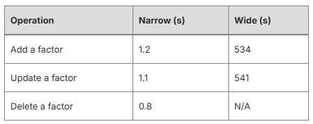
In conclusion, when dealing with 10,000 factors with data generated at 10-minute intervals, the narrow format demonstrates faster performance in terms of factor querying and maintenance, whereas the wide format is more efficient in data writing and storage optimization. In general, the narrow format stands out as the more suitable solution for storing factor data.
3.4. Test 2: Storing on SSD
In real-life situations, we often choose SSDs to store factor data instead of HDDs for better performance. In this section, we’ll store six months’ worth of factor data in both narrow and wide formats using SSDs. Then we will compare the performance of these two solutions in terms of data writing, querying, and maintenance.
Environment:
CPU: 48 cores
Memory size: 512G
Disk: 4 SSDs
Database: Single-server cluster with 2 data nodes
Writing factor data
In this test, we write 6 months’ worth of 10-min frequency factor data for 10,000 securities to the database concurrently by submitting multiple background jobs. The script used is the same as used in Test 1 (see Appendixfor full script). The test results are as follows:

The results show that wide format is faster in writing and consumes less storage space.
Querying Factor Data
In this test, we query 1 month’s, 3 months’, and 6 months’ worth of random factors of 5,000 securities in narrow and wide formats. The script used is the same as used in Test 1 (see Appendix for full script). The test results are as follows:
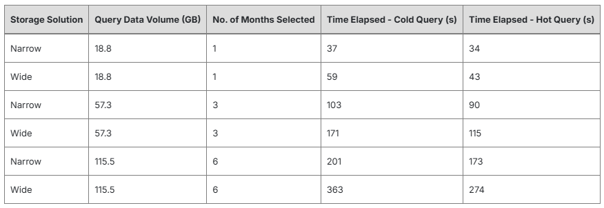
The results show that when using SSD storage, the query time for the narrow data remains lower than that of the wide data. Furthermore, as the query data volume grows, the query time increases linearly, without experiencing a significant increase in query time.
Maintaining Factor Data
In this test, we continue to use factor data spanning 1 month, 3 months, and 6 months to perform factor addition, modification, and deletion operations on each dataset. The script used is the same as used in Test 1 (see Appendixfor full script). The test results are as follows:
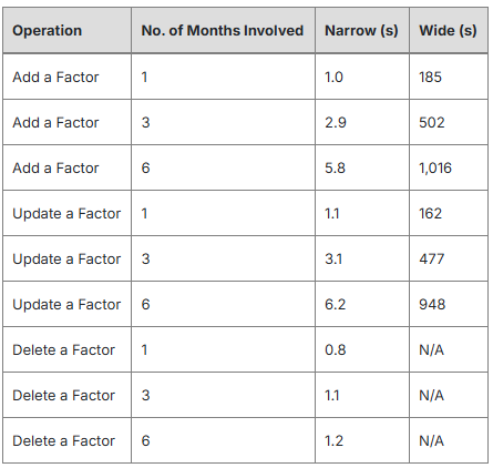
The results show that the narrow format continues to significantly outperform the wide format, and the time required for all operations also increases linearly as the data volume grows.
Throughput
As discussed in Test 1, panel data analysis in the narrow format is executed in a multithreaded manner across partitions, which consumes more CPU resources.
To evaluate whether multithreading impacts performance due to resource competition, we use 8 threads to query 1 month’s data (19GB) for 10,000 random factors across 5,000 securities in both narrow and wide formats. The results are as follows.

The results show that, with 8 concurrent threads, the narrow format’s query time increases slightly, but remains at a similar level to that of wide format queries.
In this section, we test the storage solutions with up to six months of factor data (reaching the terabyte level) on SSDs. With proper partitioning, the narrow format maintains stable performance for writing, querying and maintenance. Using 8 threads for multithreading does not significantly degrade query speeds compared to the wide format. Additionally, for the narrow format, the time required for both querying and factor maintenance increases linearly with data volume, ensuring efficient handling of massive data.
3.5. SSD Storage vs. HDD Storage
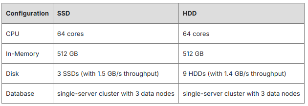
So far, we have compared wide and narrow format storage on SSDs and HDDs separately. In this section, we compare SSD and HDD storage using nearly identical system configurations as listed below. This allows us to observe the impact of disk type on performance.
Writing Factor Data
In this test, we write 1 month of 10-min frequency factor data for 5,000 securities to the database in narrow and wide formats. The script used is the same as used in Test 1 (see Appendix for full script). The test results are as follows:

The results show that with similar total disk I/O, SSDs exhibit slightly faster write speeds compared to HDDs.
Querying Factor Data
In this test, we query 1 month of 1,000 random factors for 5,000 securities in narrow and wide formats. The script used is the same as used in Test 1 (see Appendix for full script). The test results are as follows:
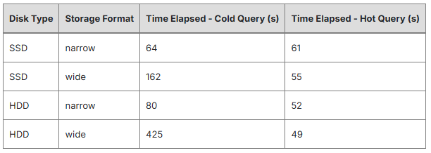
The results indicate that the performance difference between cold and hot queries is more pronounced on HDDs compared to SSDs. For both storage types, the narrow format with multithreaded querying shows more stable performance than the wide format.
Maintaining Factor Data
In this test, we test the performance of SSDs and HDDs for factor data maintenance operations. The total volume of data on disk is 186 GB in the narrow format and 166 GB in the wide format. The script used is the same as used in Test 1 (see Appendix for full script). The test results are as follows:
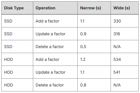
The results show that with the narrow format, both SSDs and HDDs demonstrate exhibit fast and consistent performance, taking around 1 second per operation. In contrast, despite faster speeds on SSDs, the wide format remains slower overall compared to the narrow format on both disk types.
The tests so far reveal that with equivalent hardware configurations, SSD storage demonstrates faster performance for factor data writing and cold querying compared to HDD storage. For factor maintenance, the narrow format shows little performance difference between SSDs and HDDs — all operations are executed rapidly. In contrast, the wide format shows a significant performance gap between the two disk types, with SSDs significantly faster than HDDs.
Therefore, we recommend using SSD storage to achieve optimal performance across the board for factor data storage.
4. Conclusion
In this tutorial, we compare storage formats (narrow vs wide) and disk types (HDD vs SSD) for a dataset of 10,000 factors calculated at 10-minute intervals. Performance is evaluated for data writing, insertion, modification, deletion, and querying (including concurrent querying using multiple threads).
The test results indicate optimal storage solution for this dataset is a narrow format table partitioned by month and factor name, with security ID and trade time as the sorting columns.
With concurrent queries, the performance of narrow format slows slightly due to resource competition, but it still keeps the performance gap within 5% to that of the wide format.
The recommended narrow format storage solution maintains stable performance on both HDDs and SSDs. It writes data slightly slower than with the wide format, but has advantages for factor querying and maintenance. Especially in maintenance scenarios, all operations take just a few seconds with the narrow format.
Therefore, we recommend users to store high frequency trading factors using the narrow format with thoughtful partitioning design.
Appendix
Subscribe to my newsletter
Read articles from DolphinDB directly inside your inbox. Subscribe to the newsletter, and don't miss out.
Written by
