ML Classification 3.4: Kernel SVM
 Fatima Jannet

Hello and welcome back to machine learning. Previously we learned about linear support vector machine algorithm. Today we’ll learn the kernel support vector algorithm. Let’s start
Kernel SVM Intuition
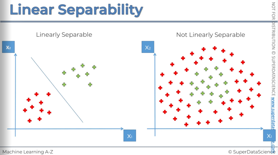
As you can recall, in the support vector machine we has a set of different observations and our task was finding a boundary line which will identify the category of any future observation. When we use the support vector machine it already assumes that the observations are linearly separable and thus helps us finding the boundary between them.
But what happens if we can’t find any boundary? For example, look at the plot at the right side. How can we possibly draw a boundary here that will separate the two categories? What are we suppose to do here? The support vector machine won’t work here.
Well,
This section is about developing an algorithm to handle situations like these, where we need to identify a class that is surrounded or in cases where you can't simply draw a line.
Mapping to a higher dimension
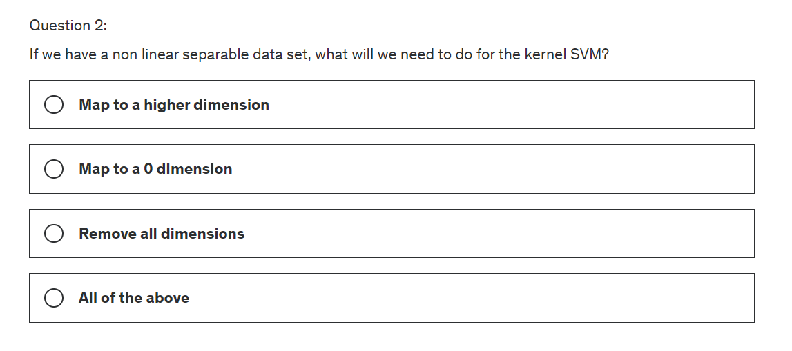
First, we will learn how to take our non-linearly separable dataset, map it to a higher dimension, and make it linearly separable. Then, we'll apply the support vector machine algorithm to build a decision boundary for our dataset and project everything back into the original dimensions. There's quite a bit to cover, so let's get started.
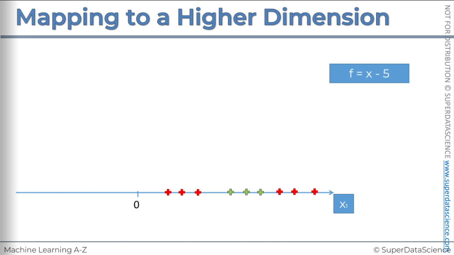
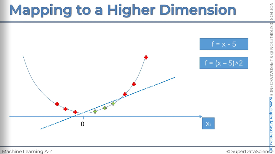
Right now, here’s a single dimension. There are observations over here. If we want to put a divider, it’d be a dot not a line cause this is a single dimension. (In a 2D space the linear separator is a line, and in a 3D space, the separator is a hyperplane) They are not linearly separable, we’ll need another dimension to fit a linear line to separate these observations. Now we’ll look for a method to increase a dimension. (It’s very magical)
Our first step to building a mapping function is to set f = x - 5
Imagine, somewhere here we got a 5 (doesn’t matter, could be any number)
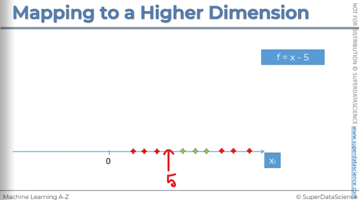
To subtract 5 from our dataset, we move everything to the left. This is what the result looks like: if you take 5 and subtract it from X, some values will become negative, while others will remain positive. The next step is to square all of these values. So, F is now equal to (X - 5) squared.
So how will that all look?
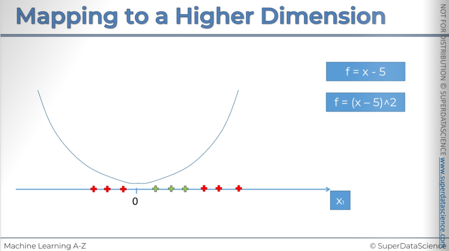
Well, basically, you'll have this squared function going through your chart, and all of these will be projected onto the function.
There you go.
So, that's what it looks like: F = (X - 5) squared.
Now, what we want to do is check that it is indeed linearly separable. And there it is—our linear separator. In a two-dimensional space, as we remember, a linear separator is a straight line. As you can see, this dataset has become linearly separable in this dimension. I know it's surprising and even a bit shocking.
This happens when you map a function. Now let’s proceed top a higher dimension.
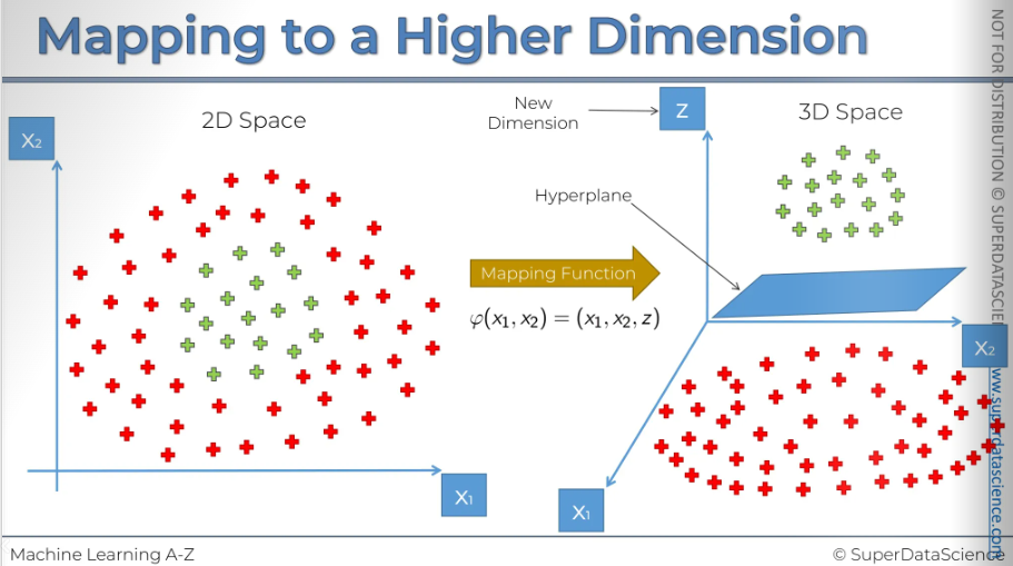
So this is our 2-dimensional space. Basically we will apply the same principle here. Here you can’t invoke the support vector machine algorithm because this is a non-linearly separable data set. But then again, we would apply some kind of mapping function. Right now we I won’t go in details what kind of function it will be. But we know and saw evidence that it works right? It applicable for the 2D, 3D space too.
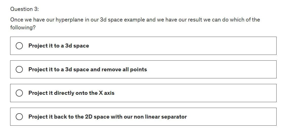
However, here we have the new dimension, which is Z. In a three-dimensional space, the linear separator is no longer a line; it's a hyperplane. This hyperplane separates the two parts of our dataset as desired. The support vector machine algorithm has helped us build this hyperplane the way we want.
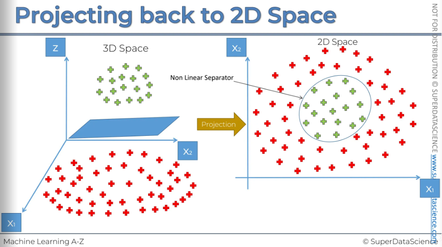
So, once we have this result, we project it back into our two-dimensional space. This gives us a circle that either encompasses or separates our classes. And there you have it, the non-linear separator.
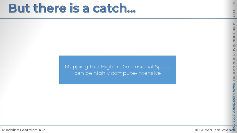
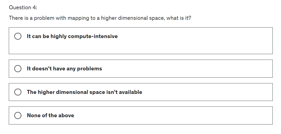
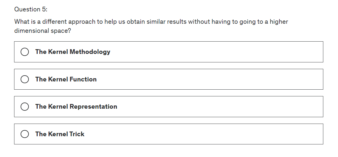
Bu there’s a problem with this algorithm. Mapping to a higher dimensional space can be highly compute-intensive. Computing to higher dimension and then getting back to the lower dimension will cause a lot of backlog, delays and issues in your computer. If the data are enormous, then it will require even more computation and processing power. And we don’t want this happen. Therefore we will explore another possibility, which is called, in mathematics, the kernel trick.
The Kernel Trick
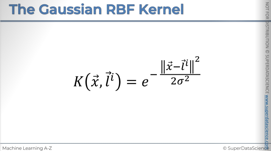
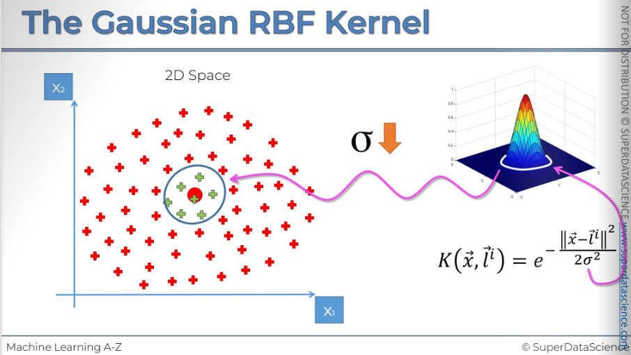
So here we've got the Gaussian/radial basis of function kernel, and those are two interchangeable terms.
K stands for kernel, it’s a function applied to two vectors. The x vector is a sort of point in our dataset and L stands for landmark (i means there can be several landmarks). And then that equals to an exponent in the power of minus the double vertical lines, mean the distance between X and the landmark squared divided by two sigma squared.
I know this might seem very confusing right now, and you're probably wondering, "This makes no sense at all. What does this even mean?" Well, let's explore this with a visual example.
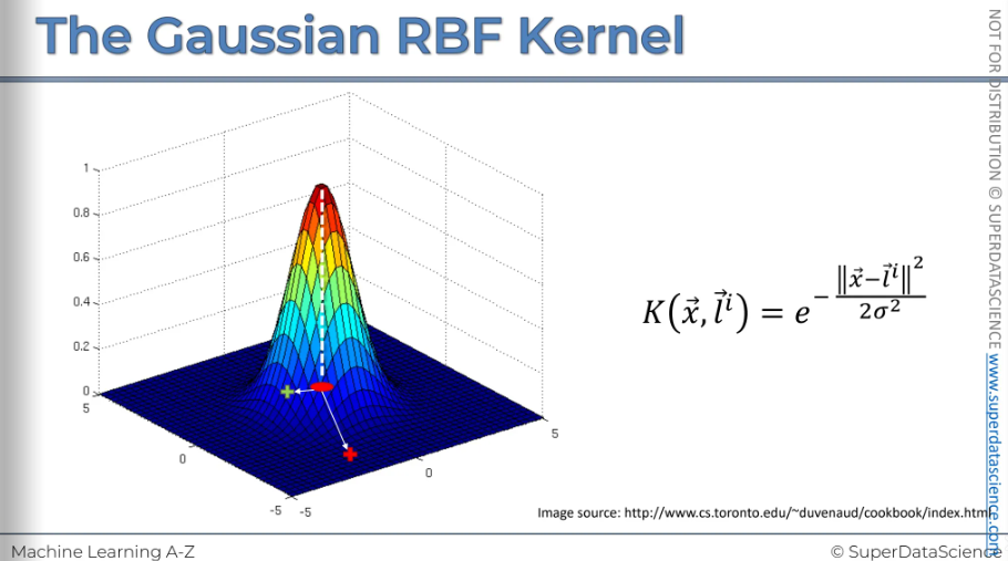
This image represents the formula. We've got L the landmark which is in the middle of this plane. In the middle we've got zero and that's where the landmark is actually located. The vertical axis represents the result we get when we calculate this for every other point on the XY axis.
Let's say we place that point here, calculate the distance to the landmark, square it, and divide by two sigma squared, where sigma is a fixed parameter. Then, we take the negative of that and raise it to the power of the exponent. This gives us the result, and that's what it will look like.
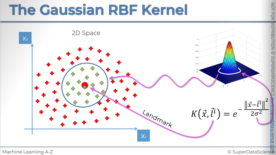
Sigma defines how wide this circumference will be.
Increasing sigma will widen the circumference.
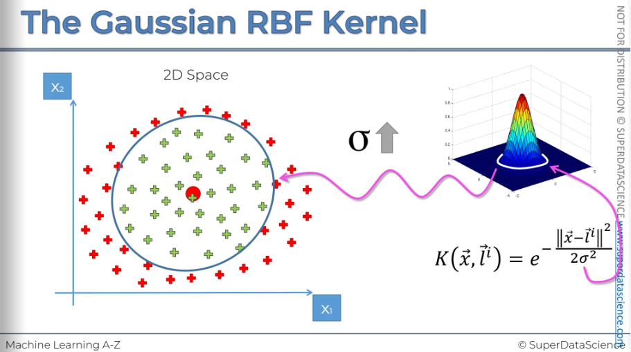
And the vice versa
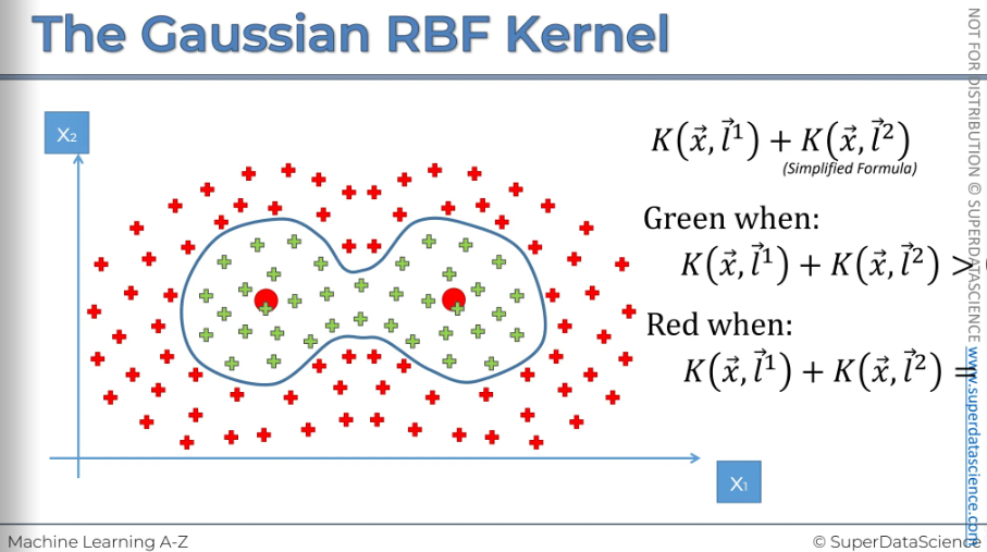
If you have more complex problem like this, add two kernels The big red points are the landmarks. Therefore you can draw a non linear boundary.
The point is assigned to the green class when this equation is greater than zero, and it is assigned to the red class when the equation equals zero. Again, this is a very simplified example; in reality, it is a bit different.
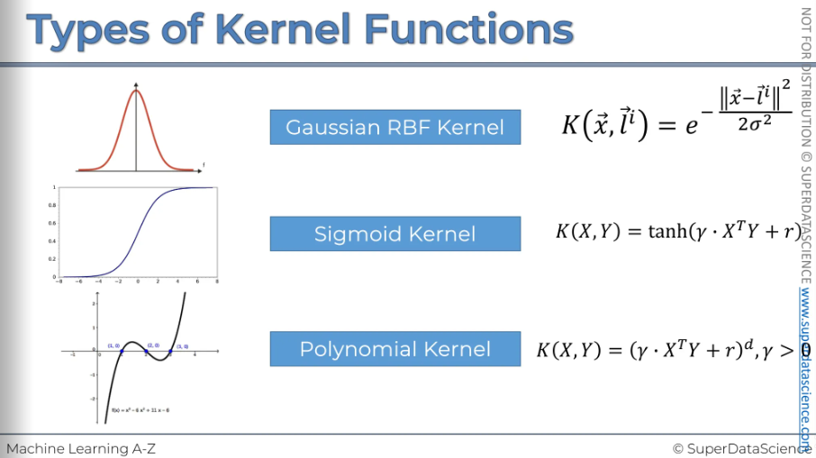
Types of Kernel Function
Gaussian formula is not the only thing used for kernel trick. There are more popular kernels too, for example: the sigmoid kernel, the polynomial kernel. The process is kinda similar too. You have to choose a landmark then proceed to your decision boundary.
Non Linear Kernel SVR (Advanced)
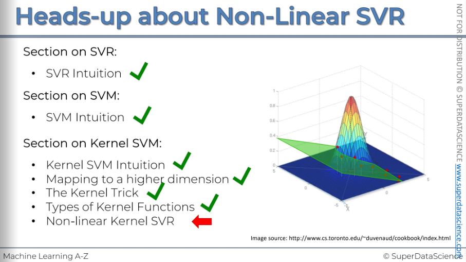
Before proceeding, please make sure that you have completed all the previous lessons on SVR and SVM kernels.
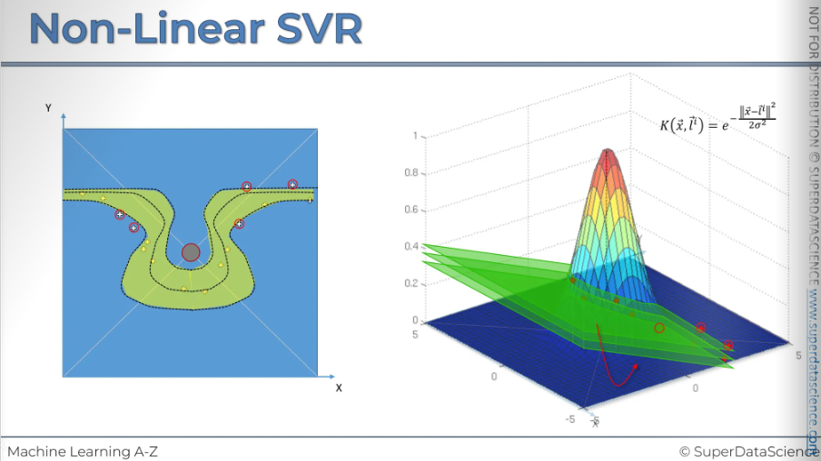
Imagine you have a data set like this(left plot) and you are trying to fit a regression model and you want to see what kind of trend line, what kind of equation is here so that you can predict what the next value is going to be.
Now you fit a regression model (right graph) but you can clearly see it’s not the right one. Maybe for some value, it’s correct but for other values it’s incorrect.

You may try something like this (left) but this also doesn’t work. You can try another (right) but this isn’t working either.

But nothing fits right? It seems like a linear regression is not a suitable fit for here. We need something else that will be appropriate for this data set.
Now here’s the things, we have to take out data to another dimension. And just for visualization purposes, we're gonna add the blue box and the red circle in middle of it. It has nothing to do with the algorithm, it’s just for visualizing purpose. Now we have take it to z dimension.

No let’s get rid of the previous view. The make a copy of it. We are going to add a kernel on it. We're gonna add the a radial basis function or the RBF. You can see our data vaguely underneath. And just to, as a reminder the formula for the RBF function is over there. So first of all, the center zero or this 0.0000 on x or Y axis projects straight into the very top. And if you, we discussed this before in the lessons, if you put (0, 0), L is the distance from the center you'll get the very top, you'll get a one. Now let's look at how these other points, the other points in our visualization will be projected onto the view. Now what happen next?
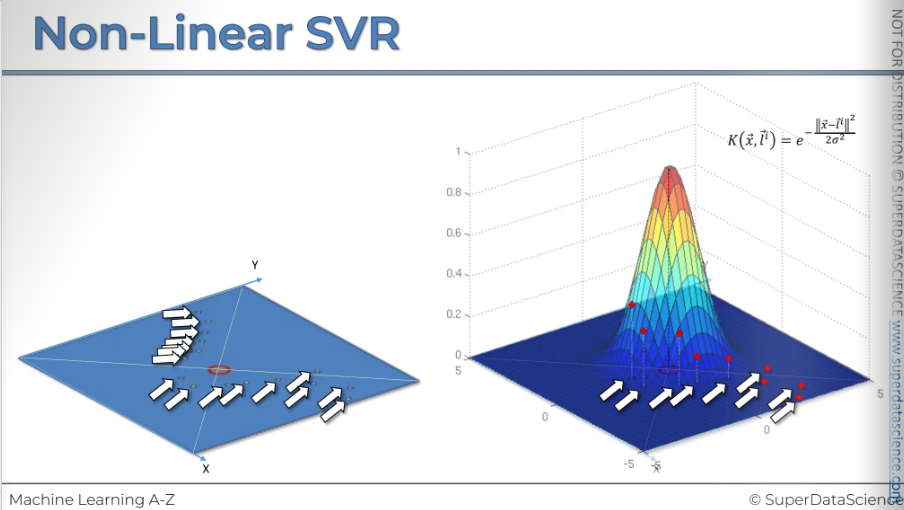
Next, in this three dimension, we need to create and run a linear model. In 2D space, linear is a straight line. But in 3D space, a linear model is a hyperplane. So now if we run a linear model it will look something like this.
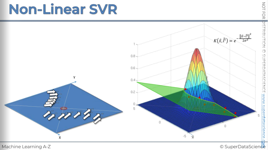
Now we want to see where does it actually cross. Where does it actually intersects our RBF function. Now, if we remove the plane, we are left with a line. Then we will reproject it back to the z dimension.
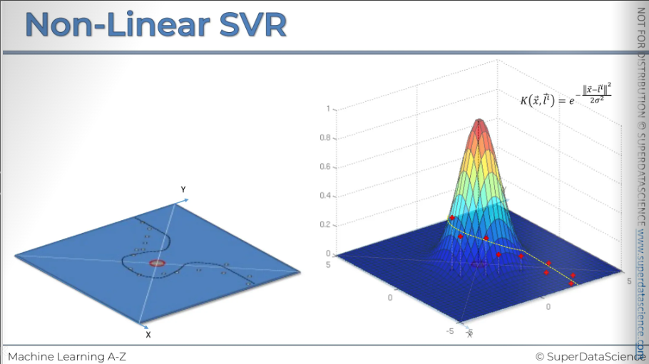
Now that’s what it will look like.
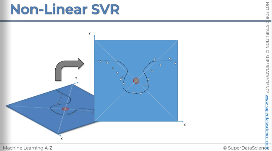
First, we have this two-dimensional plot. Now, in three dimensions, SVR works similarly to two dimensions. Instead of an epsilon-sensitive tube, we have an epsilon-sensitive space between hyperplanes. We add two new hyperplanes: one epsilon above and one epsilon below. Points between these hyperplanes won't count towards the error. The red marked points is our support vector points. The outcomes are identified/built from this view from the 3D view.
Python Implementation
Resources
I have shown how do do this in the first blog of ML.
Colab file: https://colab.research.google.com/drive/1U2p46TcDjQyYx80tQdZkiANbGTjEv8Po (copy a file)
Data sheet: https://drive.google.com/file/d/1jvnTtPStrJU5oi3_gyInitFmRyn-cSfj/view (download and add this to your colab copy)
Training the Kernel SVM model on the Training set
This is same as SVM. You just have to change the name from linear to rbf

Making the Confusion Matrix

We achieved 93% accuracy. We didn't surpass K-NN, which also had 93% accuracy, but we managed to reach our best accuracy so far.
Visualizing
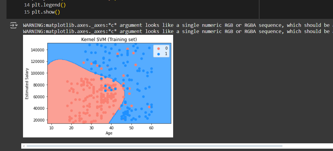
We got some amazing curves. Let’s look at them
Training set
These curves are nicely catching the observations which linear boundary wasn’t able to cancel.
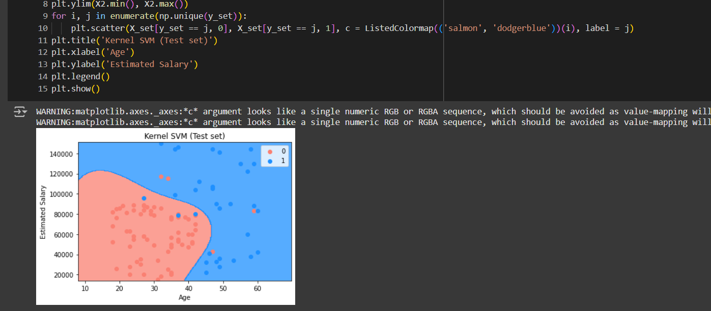
Test set
The test set looks even better. In 100 person, it got 93 of them correctly.
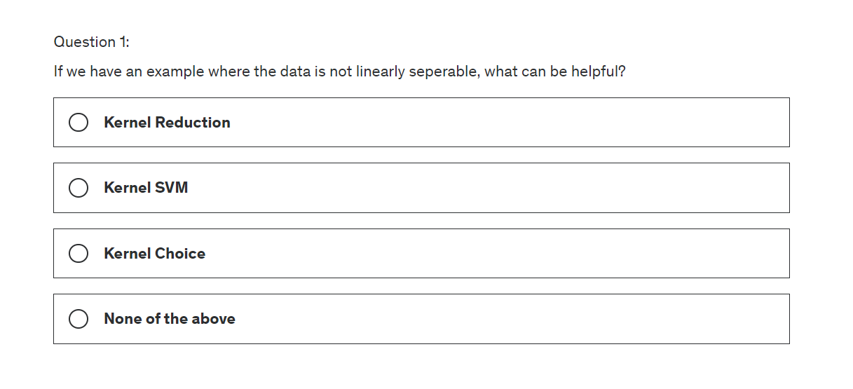
Quiz
Answer
Kernel SVM
Map to a higher dimension
project it back to the 2D space with out non linear separator
It can be highly compute-intensive
The kernel trick
Great job! You are ready to move on to the next blog Naive Bayes
Subscribe to my newsletter
Read articles from Fatima Jannet directly inside your inbox. Subscribe to the newsletter, and don't miss out.
Written by
