Enhancing GAN Stability with Wasserstein Loss and Gradient Penalty

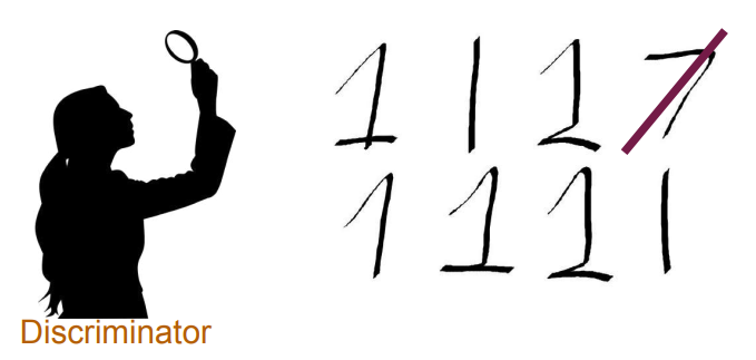
Generative Adversarial Networks (GANs) are widely used to model complex data distributions, but traditional GANs, particularly those using Binary Cross-Entropy (BCE) loss, face significant issues that hinder effective training. In this article, we’ll delve into two primary challenges with traditional GANs: mode collapse and vanishing gradients. We’ll then explore Wasserstein GANs (WGANs), which incorporate Wasserstein Loss (W-Loss), also known as Earth Mover’s Distance, as a solution to these problems, especially when combined with a Gradient Penalty (GP) to enforce a 1-Lipschitz continuity condition on the critic (formerly called the discriminator in BCE GANs). By integrating W-Loss and GP, WGAN-GP offers a powerful, mathematically grounded alternative to address mode collapse and vanishing gradients, ultimately enhancing the diversity, quality, and stability of generated samples.

This exploration draws heavily from resources available through deeplearning.ai.

---

The Challenges of BCE Loss in GANs: Mode Collapse and Vanishing Gradients

Before diving into the mathematical underpinnings of WGANs, let’s understand the challenges introduced by using BCE loss in GANs. Traditional GANs trained with BCE loss, a type of minimax loss, often encounter two major issues:

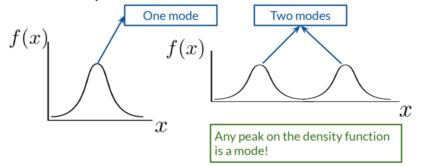
1. Mode Collapse: The generator outputs samples from a limited subset (or mode) of the data distribution, ignoring other modes. This occurs when the generator learns to exploit a weak spot in the discriminator, producing repetitive outputs that effectively “fool” the discriminator. This weakens the generative model, as it can fail to capture the true data diversity.

   

2. Vanishing Gradient: In GAN training, the discriminator outputs values between 0 and 1, which tend towards the extremes (0 for fake, 1 for real) as it improves. As these outputs approach the boundaries, gradients computed from BCE loss tend towards zero, resulting in the generator receiving diminishing feedback, which stunts its progress.

   

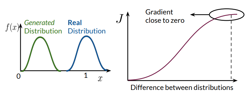
Both issues stem from the properties of BCE loss. Below, we’ll discuss the root of these challenges in the BCE framework and explore how they are mathematically addressed in WGAN-GP.

Formulating the BCE Loss in GANs

In a GAN framework, the generator ( G ) and discriminator ( D ) are in a minimax game where ( G ) aims to generate samples indistinguishable from real data, while ( D ) aims to distinguish real from fake samples.

The traditional GAN loss function (BCE loss) is defined as:

$$\mathcal{L}{\text{BCE}} = \mathbb{E}{x \sim p_{\text{data}}} [\log D(x)] + \mathbb{E}_{z \sim p(z)} [\log (1 - D(G(z)))]$$

where:

• \(x \sim p_{\text{data}}\) represents real data samples.

• \(z \sim p(z)\) represents noise input to the generator.

• \(G(z)\) represents generated data.

• \(D(x)\) outputs a probability between 0 and 1, classifying samples as real or fake.

In the BCE setup, the generator and discriminator play a minimax game:

$$\min_G \max_D \mathcal{L}_{\text{BCE}}$$

The discriminator wants to maximize \(\mathcal{L}{\text{BCE}} \) , increasing confidence in distinguishing real and fake data. Conversely, the generator seeks to minimize \(\mathcal{L}{\text{BCE}}\), aiming to produce data that the discriminator classifies as real.

Problems with BCE Loss in GANs

As training progresses, the discriminator's accuracy typically increases, leading to extreme output values (close to 0 for fake, close to 1 for real). Consequently, the gradients for the generator begin to vanish, making it difficult for the generator to improve. Additionally, the generator, aiming to "fool" the discriminator, often settles on a single mode (i.e., generating samples from a narrow region of the data distribution), leading to mode collapse.

Introducing Earth Mover’s Distance and Wasserstein Loss

The limitations of BCE loss in GANs inspired the adoption of the Earth Mover’s Distance (EMD), also known as Wasserstein Distance, as a measure of distance between distributions. This shift introduces new mathematical formulations and approaches to overcoming the issues of mode collapse and vanishing gradients.

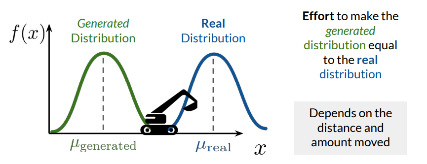
Earth Mover’s Distance (EMD)

EMD, also known as the Wasserstein-1 distance, measures the minimum effort needed to transform one distribution into another. Conceptually, EMD represents the “cost” of reshaping one distribution (generated data) into another (real data), making it a more suitable distance metric for GANs.

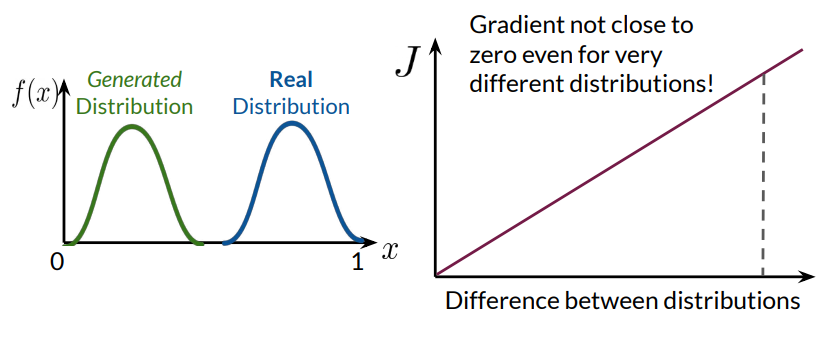
For two probability distributions \(p\) and \(q\) defined over some metric space \(\mathcal{X}\), the EMD is defined as:

$$W(p, q) = \inf_{\gamma \in \Pi(p, q)} \mathbb{E}_{(x, y) \sim \gamma} [| x - y |]$$

where:

• \(\Pi(p, q)\) denotes the set of all joint distributions with marginals \(p\) and \(q\).

• \(| \cdot |\) represents the distance metric in \(\mathcal{X}\).

In the context of GANs, the EMD between the real data distribution \(p_{\text{data}}\) and the generated data distribution \(p_g \) describes the "effort" required to reshape \( p_g\) into \(p_{\text{data}}\).

Wasserstein Loss (W-Loss)

To approximate EMD, the Wasserstein GAN (WGAN) introduces the Wasserstein Loss (W-Loss). The W-Loss function computes the difference in the critic’s evaluations of real versus generated samples. Unlike BCE loss, W-Loss avoids sharp boundary constraints (values between 0 and 1), allowing the critic to provide more informative gradients to the generator.

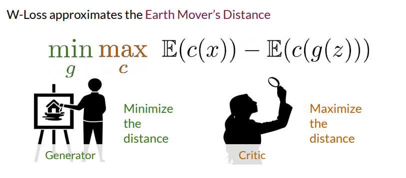
The WGAN objective is defined as:

$$\mathcal{L}{\text{WGAN}} = \mathbb{E}{x \sim p_{\text{data}}} [C(x)] - \mathbb{E}_{z \sim p(z)} [C(G(z))]$$

where:

• \(C(x)\) is the critic’s evaluation of a real sample \(x\).

• \(C(G(z)) \) is the critic’s evaluation of a generated sample \(G(z) \) .

This objective function implies that the critic aims to maximize the difference between real and fake samples, while the generator minimizes it, effectively pushing \(p_g \) closer to \(p_{\text{data}}\).

Critic versus Discriminator

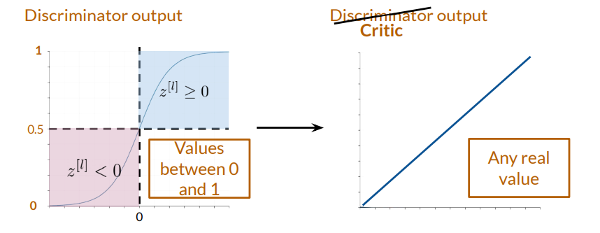
The critic in WGAN replaces the traditional discriminator. Unlike the discriminator, which outputs a probability (between 0 and 1) of real versus fake, the critic outputs an unbounded real value, estimating how “real” a sample is. This unbounded output is key to avoiding the vanishing gradient problem, as it provides a continuous measure of realness rather than a binary classification.

1-Lipschitz Continuity in WGANs: The Role of Gradient Penalty

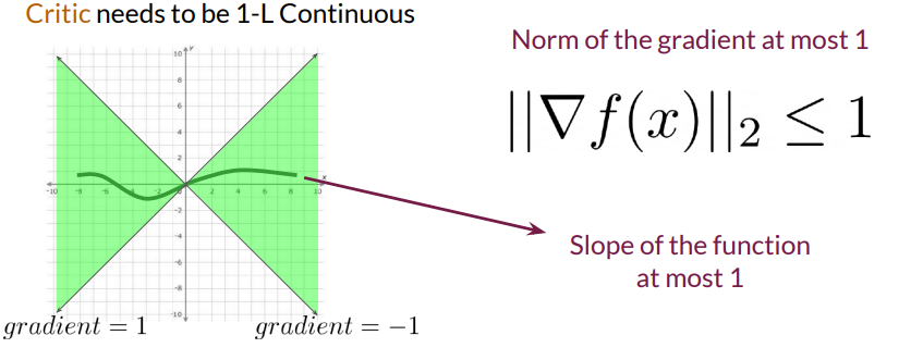
For W-Loss to approximate EMD accurately, the critic function must satisfy 1-Lipschitz continuity. A function \( f(x) \) is 1-Lipschitz continuous if, for any two points \(x_1 \) and \(x_2\), the following condition holds:

$$|f(x_1) - f(x_2)| \leq | x_1 - x_2 |$$

In simpler terms, the slope (gradient) of the function should not exceed 1 at any point, which constrains the critic’s output, stabilizing the GAN training process.

Methods to Enforce 1-Lipschitz Continuity

1. Weight Clipping:

   

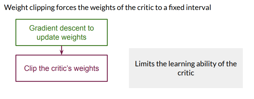
   • Description: A simple technique to enforce the 1-Lipschitz constraint by clipping each weight of the critic’s neural network to a fixed range (e.g., \([-0.01, 0.01]\)) after each gradient update.

   • Drawbacks: While effective, weight clipping limits the critic's learning capacity, potentially leading to suboptimal convergence and stability.

2. Gradient Penalty (GP):

   • Description: Instead of directly clipping weights, GP enforces the Lipschitz constraint by penalizing deviations from a gradient norm of 1, using a soft regularization term in the WGAN loss function. GP improves training stability and allows the critic to capture complex data distributions more effectively.

     

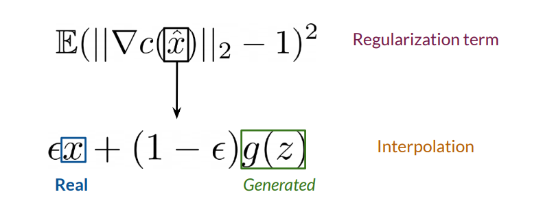
Mathematical Formulation: GP computes the gradient penalty term by interpolating between real and fake samples and measuring the critic’s gradient norm at these interpolated points. Let \(\hat{x}\) denote an interpolated sample:/m

$$\hat{x} = \epsilon x + (1 - \epsilon) G(z)$$

where \(\epsilon \sim U[0, 1]\) is a random interpolation coefficient. The GP term is then computed as:

$$\text{GP} = \lambda \mathbb{E}{\hat{x} \sim \mathbb{P}{\hat{x}} } \left[ \left( |\nabla_{\hat{x}} C(\hat{x}) |_2 - 1 \right)^2 \right]$$

Here, \(\lambda \) is a hyperparameter that controls the strength of the penalty, and \(|\nabla_{\hat{x}} C(\hat{x}) |_2 \) denotes the Euclidean norm of the critic’s gradient at \(\hat{x}\). The squared penalty encourages the gradient norm to be close to 1 without strict enforcement, making it more effective than weight clipping.

Complete WGAN-GP Objective

Combining W-Loss and GP, the final objective function for WGAN-GP is:

$$\mathcal{L}{\text{WGAN-GP}} = \mathbb{E}{x \sim p_{\text{data}}} [C(x)] - \mathbb{E}{z \sim p(z)} [C(G(z))] + \lambda \mathbb{E}{\hat{x} \sim \mathbb{P}{\hat{x}}} \left[ \left( |\nabla{\hat{x}} C(\hat{x}) |_2 - 1 \right)^2 \right]$$

This formulation maintains the benefits of W-Loss by approximating EMD, while the GP term ensures that the critic satisfies the 1-Lipschitz constraint, stabilizing GAN training.

WGAN-GP: A Solution to Mode Collapse and Vanishing Gradients

WGAN-GP addresses the limitations of BCE loss in GANs through W-Loss and GP, yielding several advantages:

1. Reduced Mode Collapse: By minimizing the Earth Mover’s Distance, the generator is encouraged to explore the entire data distribution, thereby reducing the likelihood of collapsing to a single mode.

2. Elimination of Vanishing Gradients: The critic’s unbounded output allows the generator to receive meaningful feedback even as the critic improves, maintaining effective gradient flow throughout training.

3. Improved Training Stability: The 1-Lipschitz constraint, enforced via GP, stabilizes the critic’s behavior, enabling more balanced updates and reducing the likelihood of training instability.

Conclusion

The adoption of Wasserstein Loss with Gradient Penalty represents a major improvement in GAN architecture, addressing the key challenges of mode collapse and vanishing gradients that commonly occur in BCE-based GANs. By approximating Earth Mover’s Distance with W-Loss and enforcing 1-Lipschitz continuity via GP, WGAN-GP offers a mathematically rigorous approach to generating more diverse and high-quality samples.

For those interested in further exploring GAN advancements, additional resources are available on deeplearning.ai.