ML Classification 3.5: Naive Bayes
 Fatima Jannet
Hello and welcome back to the blog of machine learning. Today we will learn about Bayes theorem. Our main focus for this blog is on naive but we can’t proceed to it without Bayes theorem so here it is.
Question Why is this algorithm called the native base algorithm?
The answer is that the Bayes theorem requires some independent assumptions, and it is the foundation of the Naive Bayes machine learning algorithm. This algorithm also relies on these assumptions, which are often not correct. Therefore, it's somewhat “naive” to assume they will always be correct.
Bayes Theorem
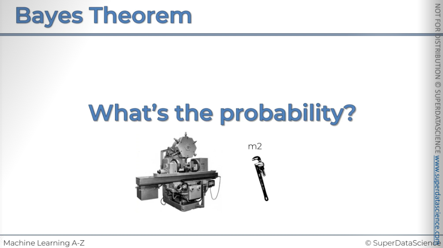
We have spanners to illustrate the theorem. This way, whenever someone mentions Bayes Theorem, you'll think of a spanner and remember what you've learned.
Let's say we're in a factory with two machines producing spanners. Both machines work at different rates but make the same spanners. The spanners are marked, so we know which machine they came from: the top ones from machine one and the bottom ones from machine two.
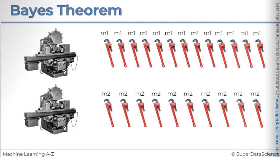
And then at the end of the day we've got a whole pile of these spanners and the workers go through them.
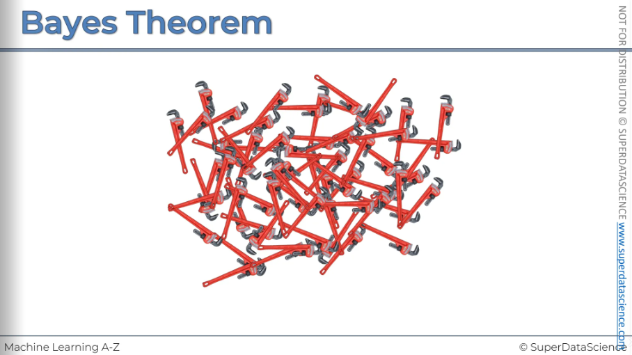
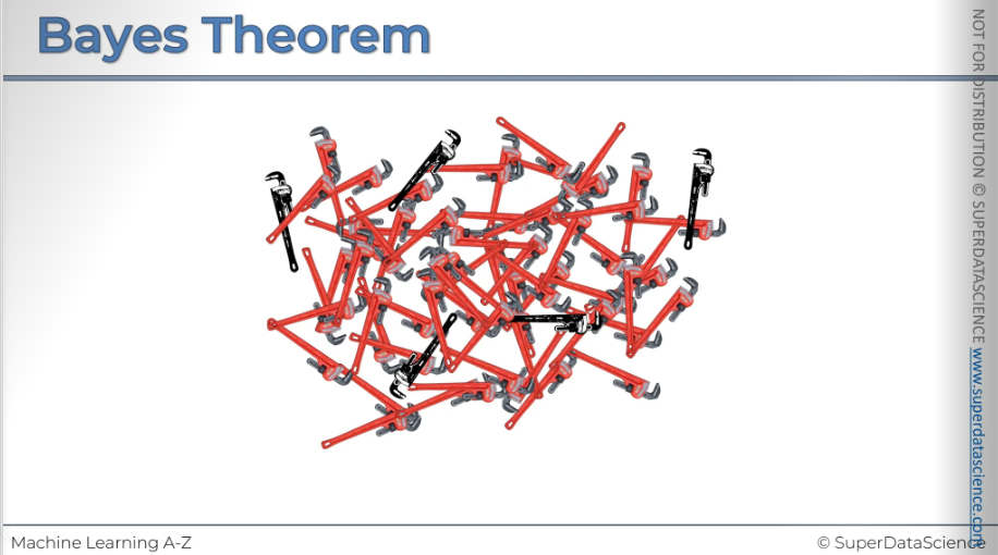
And their goal is to pick out the defective spanners (here we can see that there's a couple of defective spanners hiding among the pile, the black ones)
Our task is to find out what's the probability of machine to producing a defective spanner.
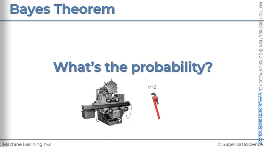
If you take a random spanner produced by machine 2, what is the probability that that spanner is defective.
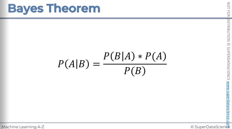
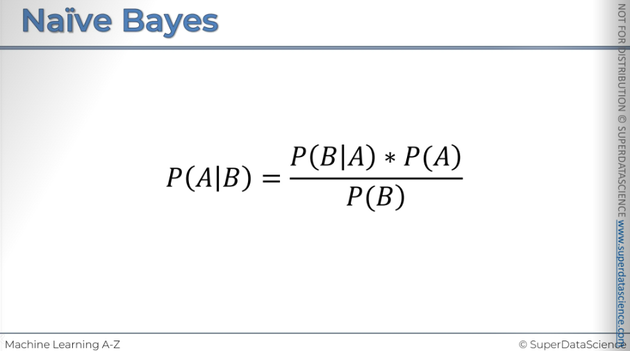
The rule or the mathematical concept that I'll be using to get that probability is called the Bayes Theorem. Here's a mathematical representation of it.
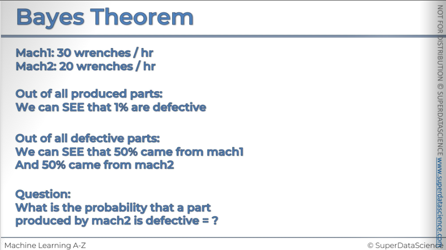
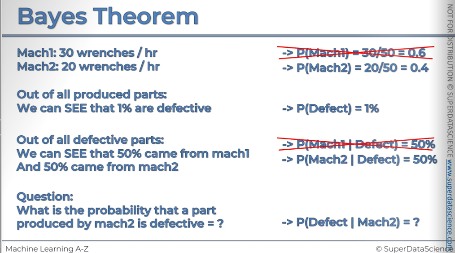
But to calculate the probability, some information is given to us already. Let’s look at these infos (By the way trenches and spanners are the same thing)
Machine 1 produces 30 wrenches/hr and machine 2 produces 20 wrenches/hr. Out of all of the produced parts we can see that 1 percent are defective. Also, we can see that out of all of the defective parts 50 percent came from machine 1 and 50 percent came from machine 2. So this is just the defective parts. Now the question is what is the probability that a part produced by machine2 is defective?
So how do we put all that information together to get the answer to this question? That's what Bayes Theorem helps us do.
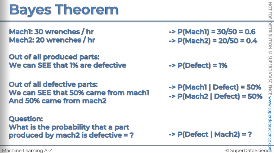
So let's have a look at how we can rewrite this information in more mathematical terms.
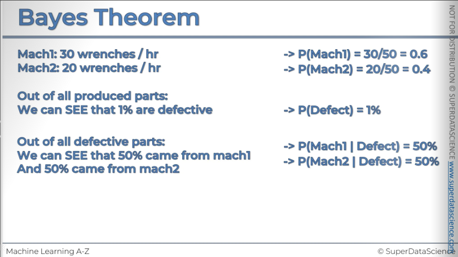
Both of the machines produces total 50 wrenches per hr.
SO, P(Mach1) = 30/50 = 0.6
P(Mach2) = 20/50 = 0.4
P(defect) = 1%
P(Mach1| defect) = 50% [probability of mach1 given that defected]
P(Mach2| defect) = 50% [probability of mach2 given that defected]
Question: P(defect|Mach2) = ?? [probability of defect given that mach2/the likelihood of it being defected knowing that it came from mach2]
As we are working with mach2, we don’t need the information of mach1. We can get rid of them.
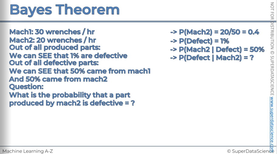
Now let’s write the bayes theorem for it (followed by the formula)
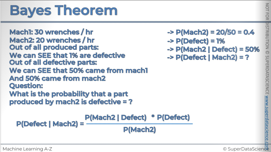
The probability of a defective part given it came from machine 2 is calculated as follows:
Start with the probability of a part being defective.
Multiply by the probability that a part came from machine 2, given it was defective.
Divide by the probability of parts coming from machine 2.
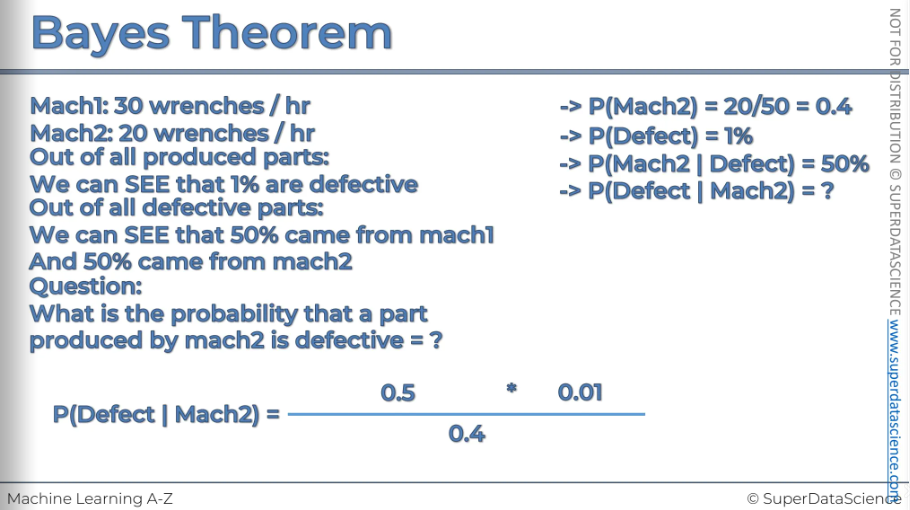
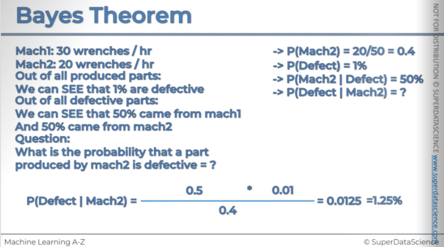
So as you can see we convert all this information that we knew about the process and got our result.
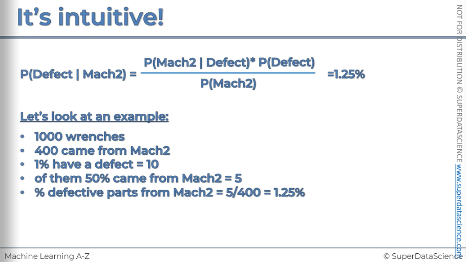
Now let's move on to the intuition the stuff. Let’s say
we have 1000 wrenches
Out of them, 400 came from mach2
1% have a defect which is 10 out of 1000
Exactly 5 of those defects came from mach2 (this line is us performing the P(mach2|defect)
So % of defectives from mach2 is 1.25%
These logical steps we took are exactly the same as Bayes' Theorem. The only difference is that we looked at a specific example with a thousand wrenches. As you can see, Bayes' Theorem is very intuitive, so we won't even delve into the mathematics of how it's derived.
This is about understanding it intuitively, so as long as you remember the mathematical representation of Bayes' Theorem, it makes sense what it helps us calculate.
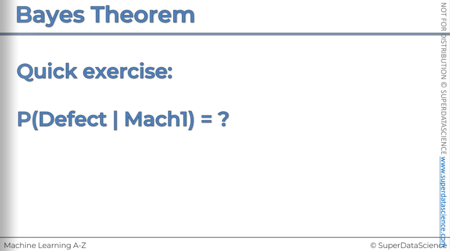
This is a handy exercise, do it yourself at home.
Naive Bayes Intuition
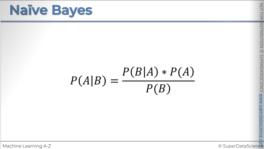
Here we have Bayes' Theorem, which we discussed right now. By now, you should be comfortable with how we'll use it to create a machine learning algorithm.
Well let's have a look here we've got a data set. So it has two features. It has x1 and x2. This graph represents observations of peoples by their salary and age. We have 30 people here on this chart.
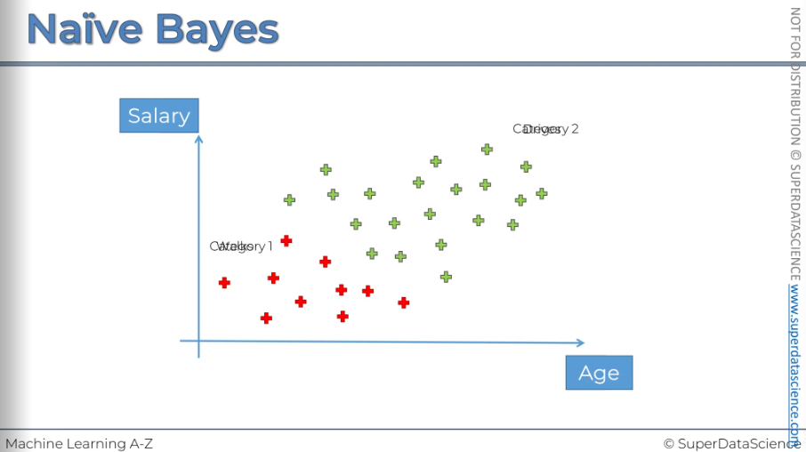
Red: that person walks to work
Green: that person drives to work
How do we classify a new data point?

We need a plan because this approach is complex. We'll break it down into steps that are easy to understand.

So our plan of attack we're going to take the Bayes Theorem and apply it twice.
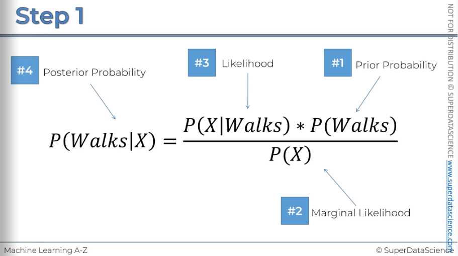
First, we'll use Bayes' Theorem to find the probability that this person walks, given their features. Here, X represents the features of that data point.
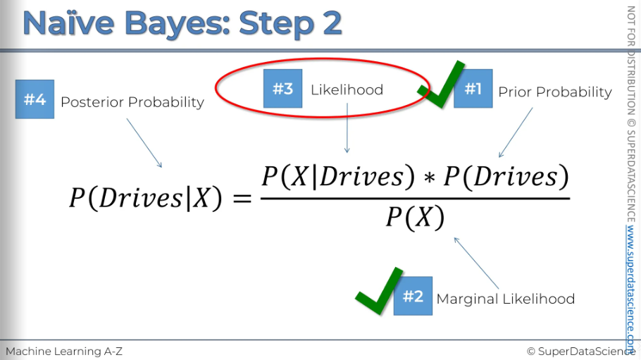
Step two: calculate the probability that someone drives, given the features X of the new data point.
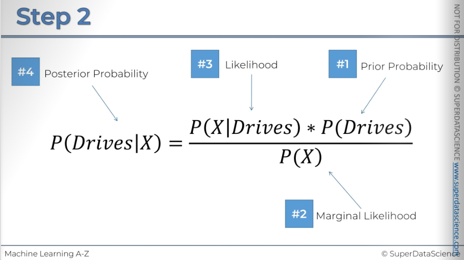
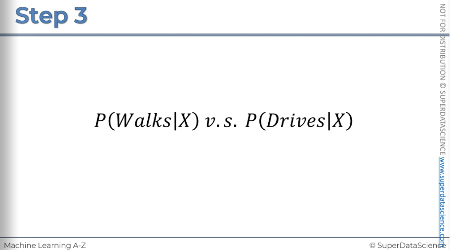
Finally, we'll compare the probability that someone walks given features X with the probability that someone drives given features X. Then, we'll decide which class to assign the new data point to.
#1: We're going to calculate the probability that somebody walks (just the overall probability)
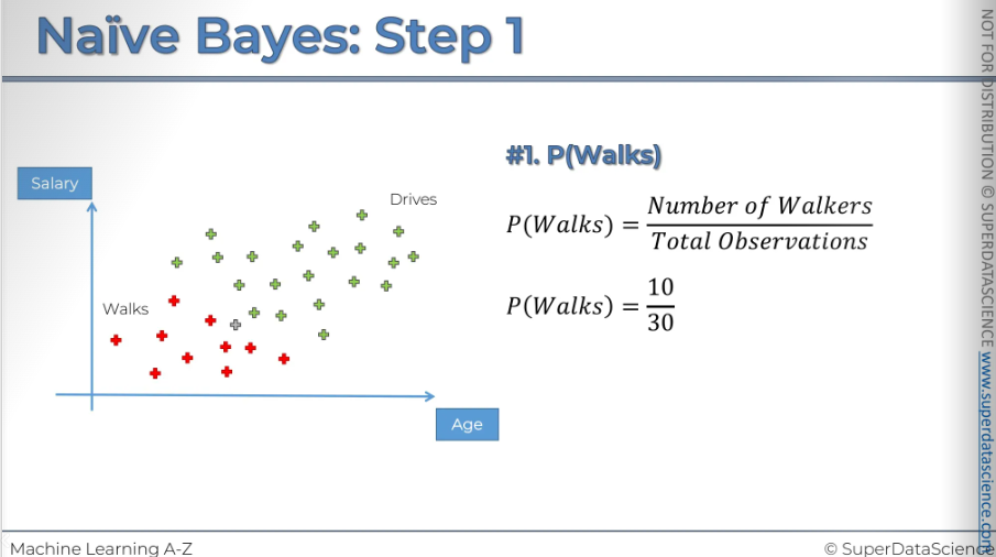
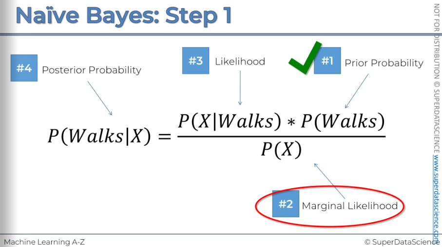
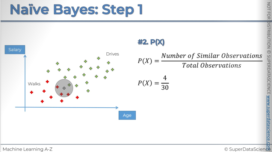
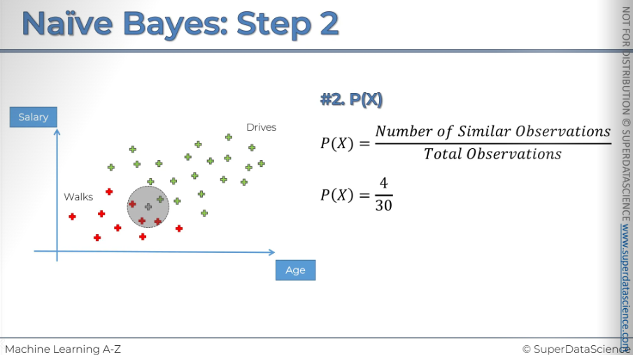
#2: Now we will calculate the margin of likelihood. First, select a radius and draw a circle around the new observation. The radius choice is up on you. Now, remove the new observation from the circle and what you are left with are the observation which we are going to deem to be similar in terms of features to the new observation we have.
(P of x tells us the likelihood of any new random variable falling inside the circle.)
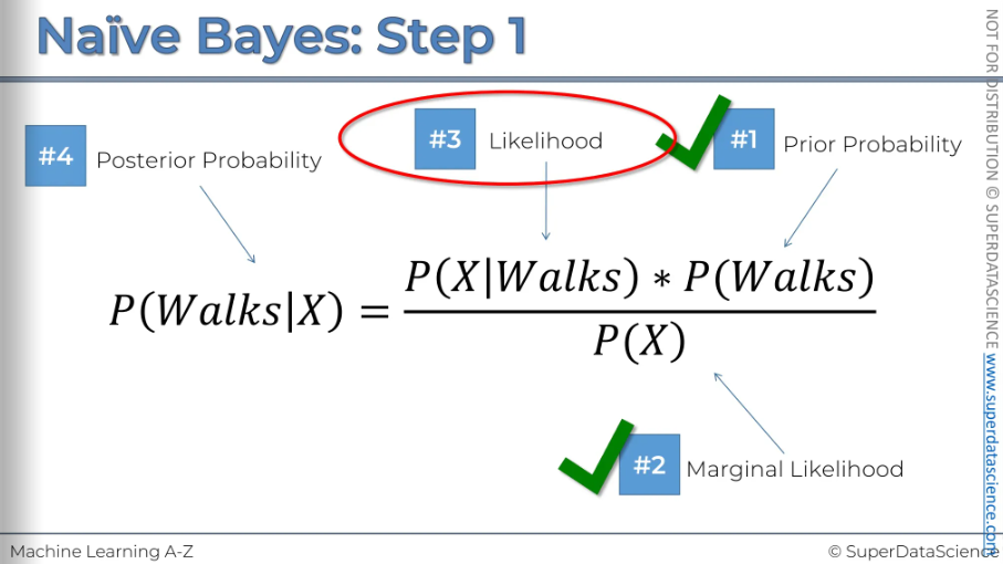
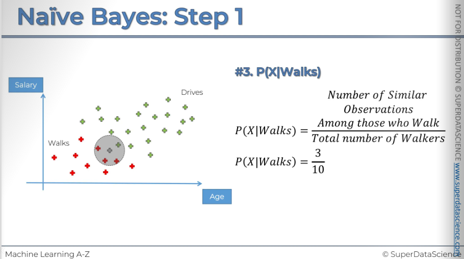
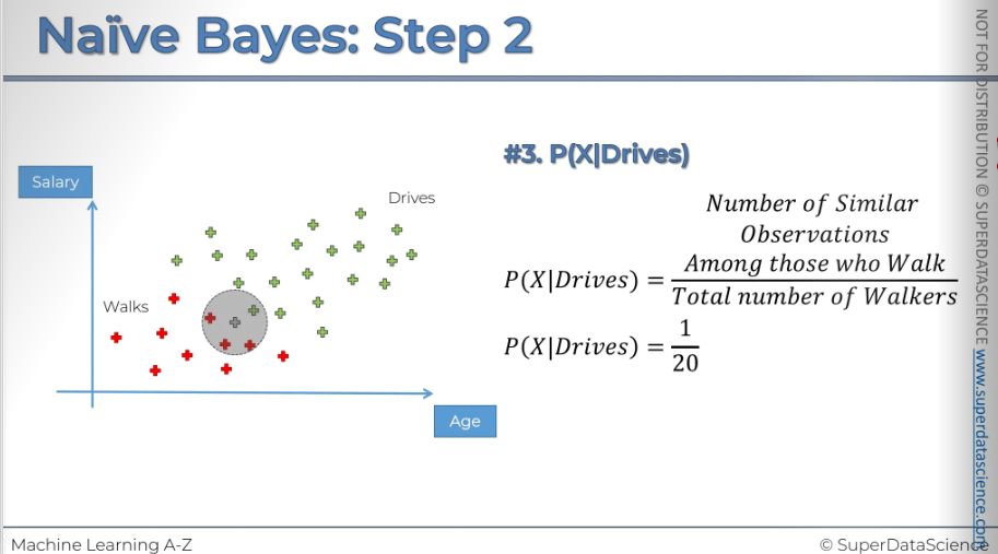
#3: We need our circle of the same radius. So basically what is the likelihood that a randomly selected data point from this circle given, (this vertical line means given that) that person walks to work. The other way to think about this is we're only working with people who walk to work. So we only need to focus on the red dots for now.
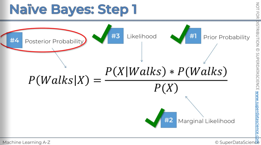
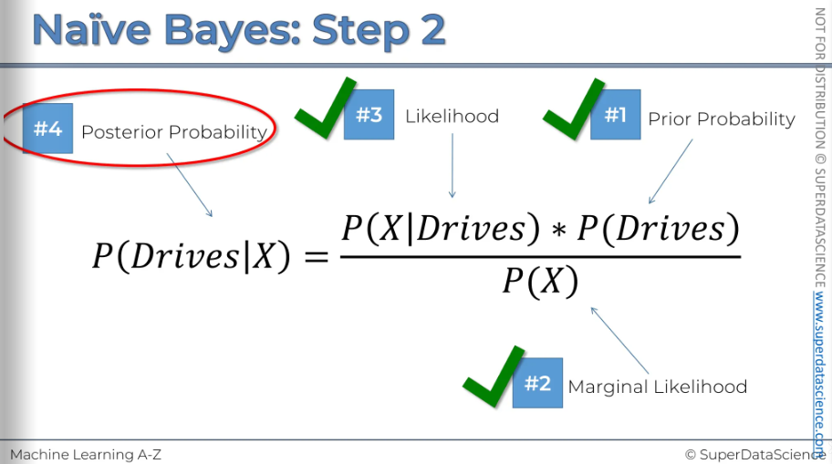
#4: Now that we have all our probability, it’s time for plug them all in.

So if we calculate that, it give us 0.75, 75% is the probability that somebody that we put into the place where we're putting x is should be classified as a person who walks to work.
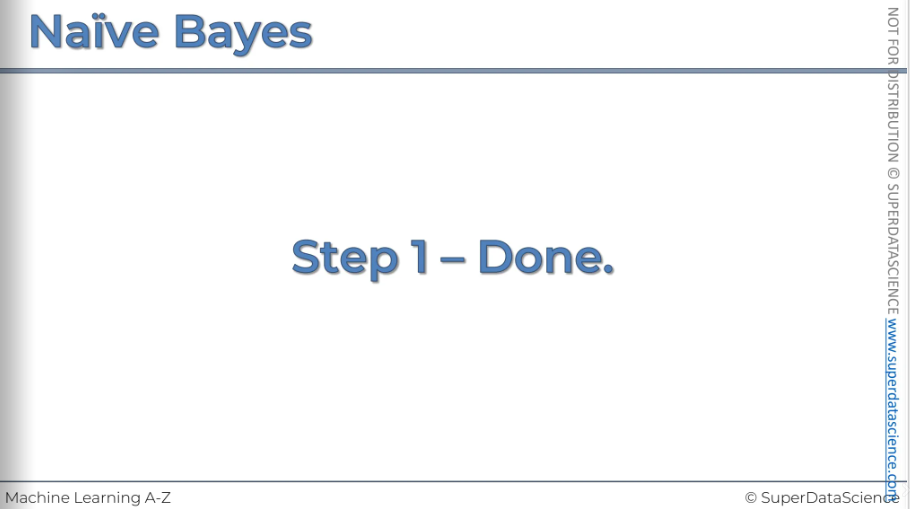
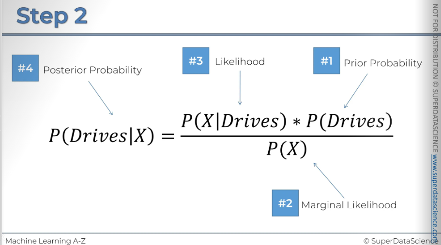
Now we will again apply the bayes theorem. Kindly do it yourself.
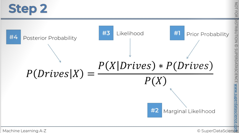
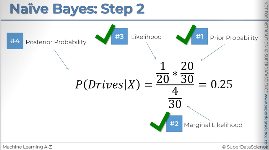
This is the result. So the probability of somebody who exhibits features X being a person who drives to work is 25%
Step 3: Compare the probabilities
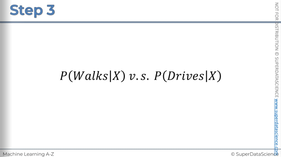
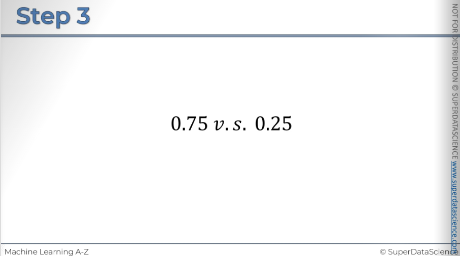
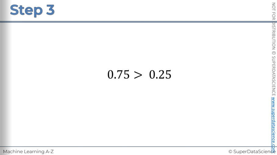
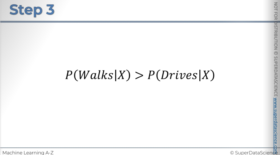
It's most likely that the new observation is a person who walks to work.
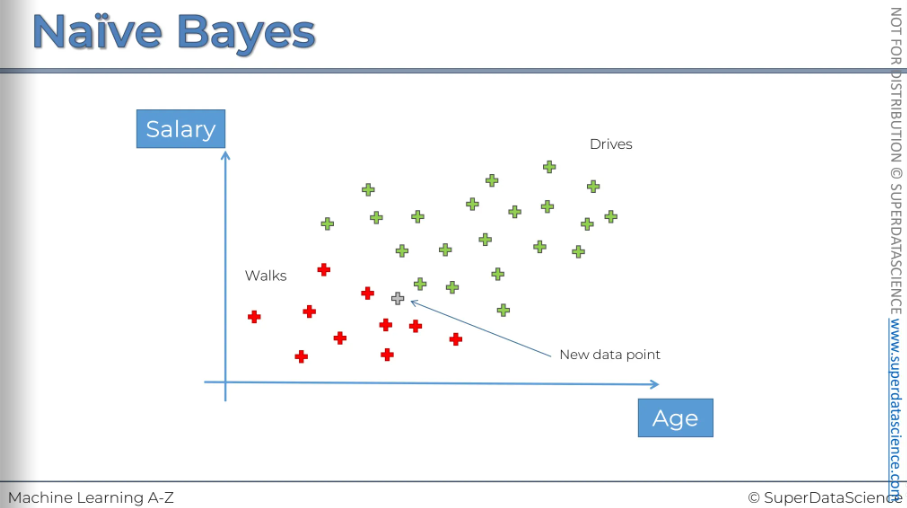
So, there's a 25% chance the person drives to work, but a 75% chance they walk. Therefore, we'll classify this point as a person who walks to work.
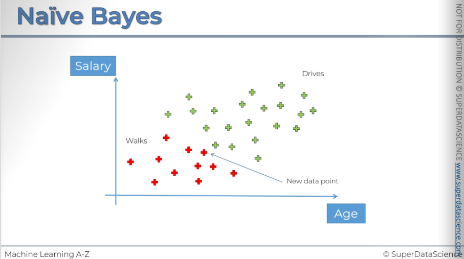
Naive Bayes Intuition(Solution)
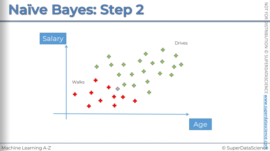
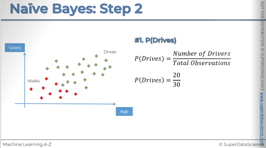
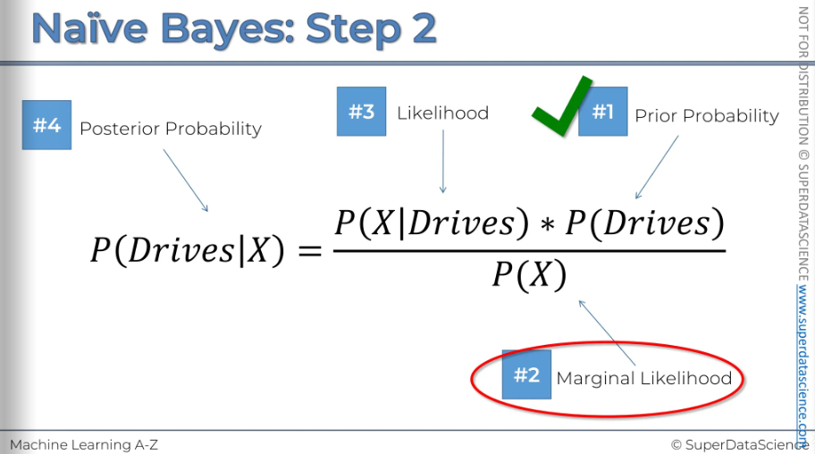
Here are the steps for applying Bayes' theorem for the second time, which I asked you to do yourself. Please take a look at these slides.
Python Implementation
Study Material
Colab file: https://colab.research.google.com/drive/1MrjCPaZ3_Vmoh3RU1QH5MVg7x9nfSZCT (save a copy in drive)
Data sheet: https://drive.google.com/file/d/1ywrni81ET6RzCnSvOQNZhHZbNdZrcQjF/view (download and add in your copy)
Let’s see if naive bayes can beat our best accuracy so far which was 93%
Training the Naive Bayes model on the Training set
To do this, you have a few options. You can type directly into the search bar of Google or Bing, or you can explore the Naive Bayes class in scikit-learn. I recommend trying the second option because it will help you become more familiar with the API, and the more you know it, the better.
In the intuition we used gaussian so it would be-


Predicting a new result
This is the predicted result for the first customer, indicating whether they bought a car or not, which our algorithm predicted correctly. Inside is his salary.

Making the Confusion Matrix
Can we beath the accuracy of 93% from both K-NN and kernel SVM??

And no we couldn’t. It beats logistic regression by 1%
Visualising the Training set results
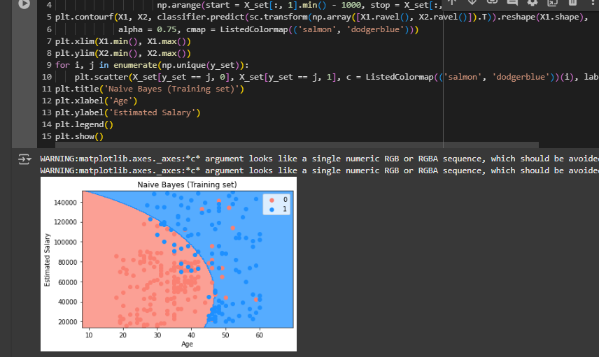
This curve is way to more smooth that's why we couldn’t get much accuracy. These errors were correctly classified by kernel svm
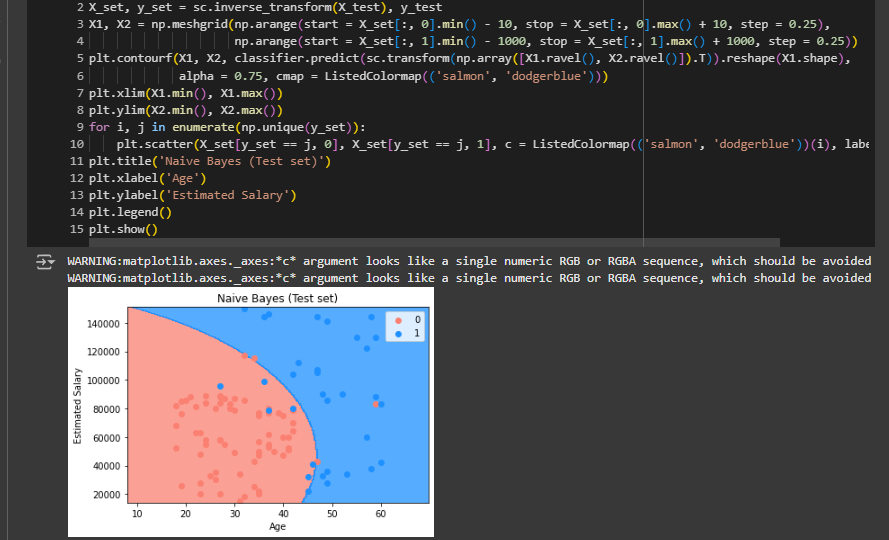
Visualising the Test set results
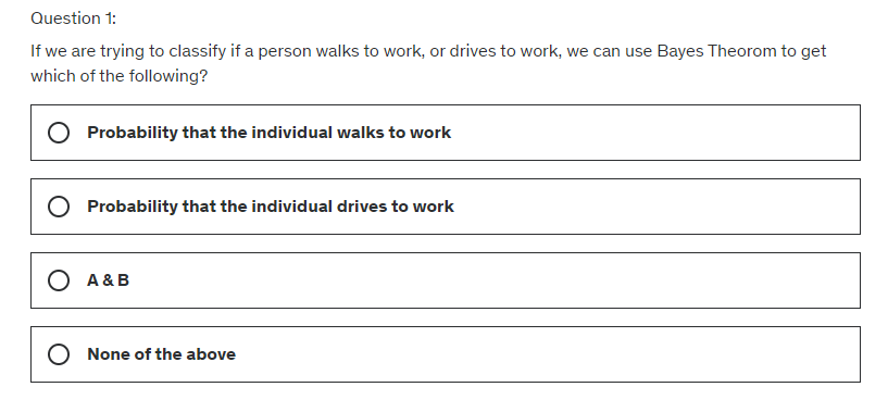
Quiz
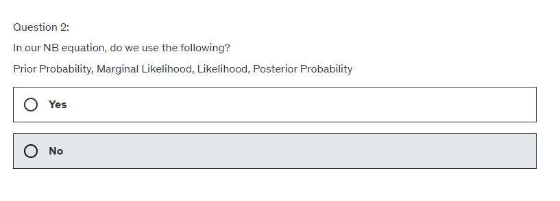
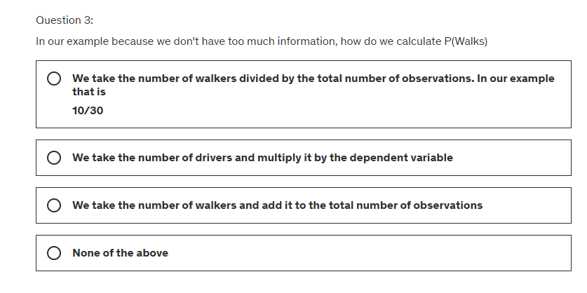
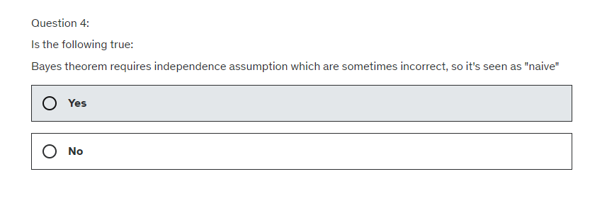
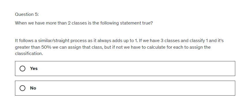
Answers
A and B
Yes
We take the number of walkers……….that is 10/30
Yes
Yes
Subscribe to my newsletter
Read articles from Fatima Jannet directly inside your inbox. Subscribe to the newsletter, and don't miss out.
Written by
