Machine Learning : Transfer Learning & Fine tuning (Part 40)

There is an image classification, global competition called image Net.

And companies all around the world are making massive, complex CNN architectures to win this competition. If you thought our neural networks were complex.

Let's take a look at this one. The network on this slide is called Inception Net. It is made by Google specifically for the image net competition. All of our networks were trained in a few minutes or even a few seconds. But these kind of architectures companies are training on hundreds of GPUs for many weeks.

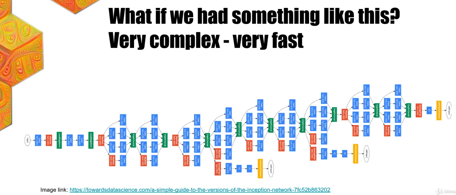
You may think at this point that these networks are just useless for everyday tasks and those resources are just thrown away for a competition. But in reality, the real power of these networks come with transfer learning.

The transfer Learning is a technique where we use a pre-trained model from an image net to perform great on a custom task.

Custom task can be anything. In our case, it will be dogs versus cats classification. This base model is the Pre-trained model on the image net dataset. It could be the inception and there is a Mobilenet Vgg 16, Vgg 19 and many more. There is a lot of pre-trained models that we could use. In this case we decided for mobilenet.

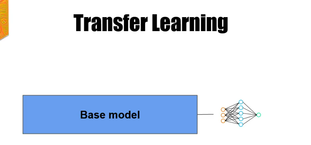
This is all great, but how to change the Pre-trained model for the custom tasks such as binary classification between cats and dogs?

When we define the Base model, we deleted a few last layers from it. That are designed specifically for the image net classification. The name of that top part of the CNN is called Head.

We use the whole Base model until its head and change the head with a custom network or the custom head for the custom task. And now we have the base model with the custom head.

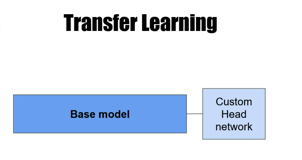
And the last thing that we have to do is to freeze the whole base model. When performing transfer learning.

Our Base model was trained on a dataset such as Image Net and its weights are learned. We don't touch them anymore. The only part of the network that is trained is the custom head part.

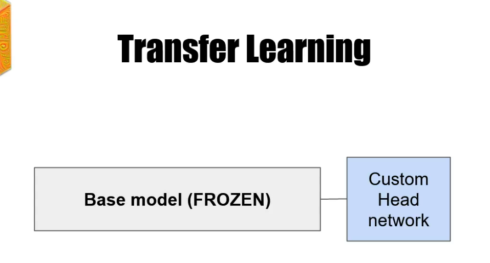
But there is one more technique that we need to discuss and that is fine tuning. Fine tuning is more suited for bigger data sets. Sometimes when the custom data set is pretty different from the imagenet data set, we need information about it in the base model as well. In the fine tuning, we still define a custom head, but we don't freeze the whole base model. We freeze only the beginning of the model

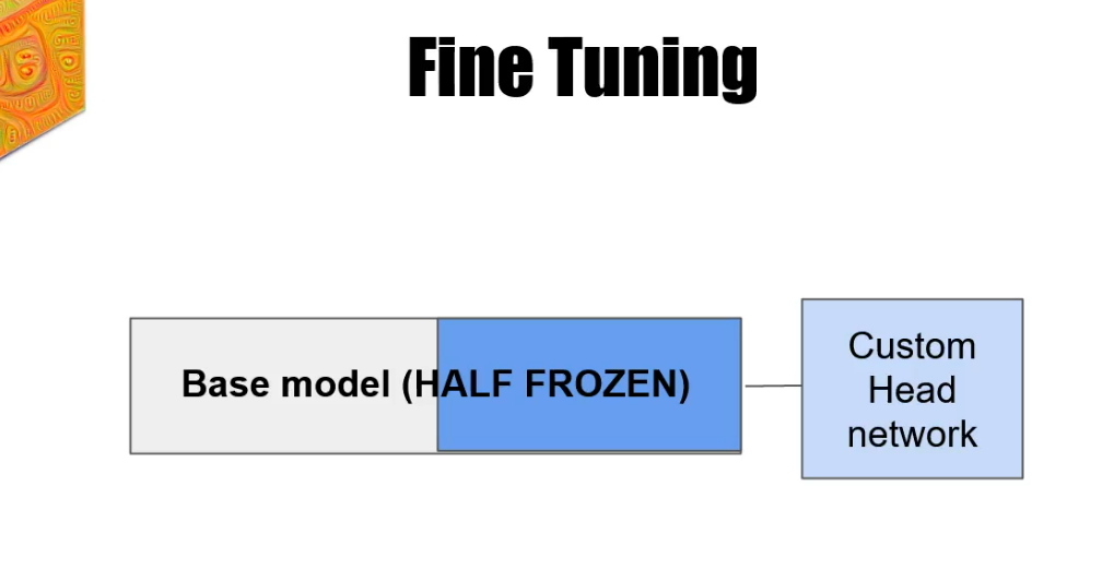
and the rest of the layers are unfrozen and ready to be changed according to the custom data set.

When to use a model or fine tuning or transfer learning?

If we have a large and different data set, train the whole model.

And when we have a large and similar data set to the one that our Bayes model was trained on, use fine tuning. Then in the case you have a small and different data set, use the fine tuning again. And finally, if you have small and similar data set, use transfer learning.

Let’s do transfer learning!

The dataset contains only two classes cats and dogs. At the first glance, the task may look very simple.

We as humans can quickly tell what a dog is and what a cat is, but that is not that obvious for computers.

Both classes have very similar features eyes, ears, fur tails and even the environment is very similar. If we were to create a custom architecture for this task, we wouldn't achieve more than, let's say, 75, maybe 80%.

And our goal is to pass 95% and get almost state of the art results on this data set by using transfer learning technique alone.

Let’s install Tensorflow and other dependencies

!pip install tensorflow

!pip install tqdm

Let’s download the dataset from the link (https://storage.googleapis.com/mledu-datasets/cats_and_dogs_filtered.zip) and save it in the current directory (./) with a name (cats_and_dogs_filtered.zip)

!wget --no-check-certificate \

https://storage.googleapis.com/mledu-datasets/cats_and_dogs_filtered.zip \

-O ./cats_and_dogs_filtered.zip

Let’s unzip the file (cats_and_dogs_filtered.zip)

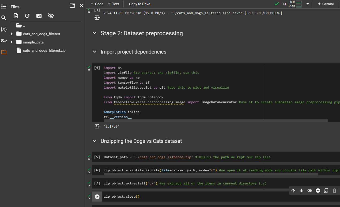
Now we have cats_and_dogs_filtered in the same location.

Building the model

IMG_SHAPE = (128, 128, 3)

Here, 128,128 for pixel size (height*width) and for colors, using 3 (red, green blue)

We are using MobileNetV2 which is a small model

base_model = tf.keras.applications.MobileNetV2(input_shape=IMG_SHAPE, include_top=False, weights="imagenet")

include_top can be TRUE Or False as we will set our custom head.

name of the dataset where the model was trained one. For us, it was imagenet

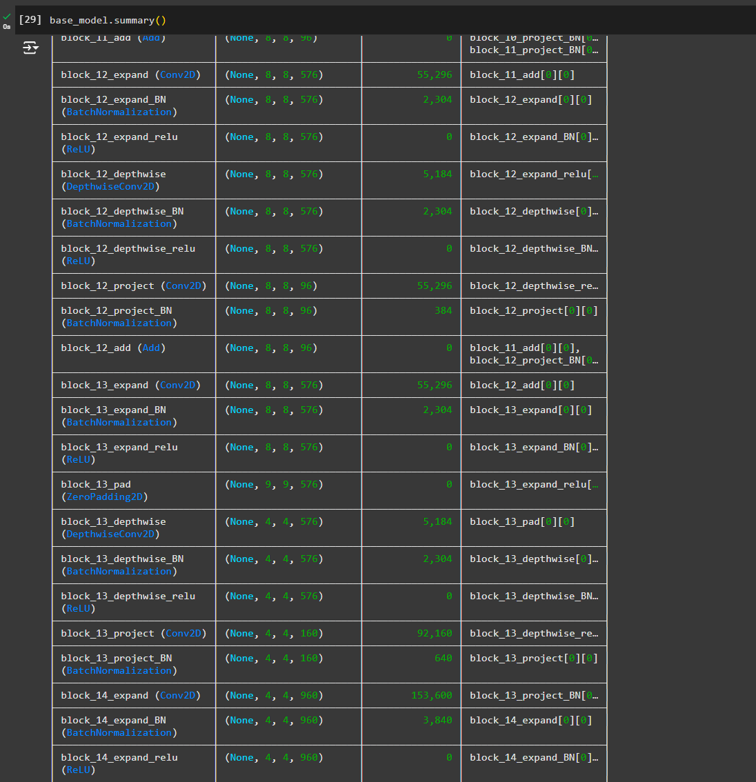
If we check the summary, we can see the model is huge!!

Freezing the base model

When you try to train your model for a specific task and you don't freeze the base network, it is going to change its initial weights as well.

And that is not what we want.

We want to take those learned features on the image net, for example, and apply them on a custom task and only train custom layers that we are going to add on top of this Base network.

To achieve this, we are going to freeze all layers in our Bayes network and only train a few layers that we are going to add.

base_model.trainable = False

Custom Head

In the previous task, we have frozen our Base network and now it's time to define our custom head on top of it.

The custom head is always designed for a task that you're trying to solve. In this case, it is classifying between cats and dogs.

To define a custom head, The first thing to do is to check what is the output size from the Base network.

base_model.output

And based on that information, we can see how many layers, if any, should be added to the custom part of the network.

As you can see, the output from our Base network has the size of 4 times, 4 times 1280. The size is not very suited for the output layer of the custom head. There are a few approaches that we can take to handle this problem:

1) As always, we could use the flattening layer to convert or reshape our output to vectors, but in this case we would have far too big vectors for our custom part of the network.

2) The other better solution in our case is to use “global average pooling layer”. We haven't discussed this layer before, but the concept is very similar to the max pooling layer that we used all across the CNNs.

The “global” word means that it's going to take the whole input instead of processing parts of it at the time. It reduces the input size significantly.

The second part of the name is “average”. Instead of finding the most significant value what Max pooling is doing, this layer takes an average of all numbers in an input.

global_average_layer = tf.keras.layers.GlobalAveragePooling2D()

Pass it the input which is the base_model.output in our case

global_average_layer = tf.keras.layers.GlobalAveragePooling2D()(base_model.output)

Now if we check the size, we can see

(None, 1280)

The only thing left to do is to define our output layer or prediction layer. Let's write prediction layer equal to tf.keras dot dense and let's provide all arguments to it.

prediction_layer = tf.keras.layers.Dense()

As we have cats and dogs (2 labels), we can use 1 neuron, Also we use sigmoid activation for binary classifications

Input to this layer will be global_average_layer

prediction_layer = tf.keras.layers.Dense(units=1, activation='sigmoid')(global_average_layer)

Final model combining with custom head

As we are connecting models, we will use Models instead of Sequential model

model = tf.keras.models.Model()

So write base_model.input and for the output, set our prediction layer.

model = tf.keras.models.Model(inputs=base_model.input, outputs=prediction_layer)

And that's basically it. We have combined two networks from our base model.

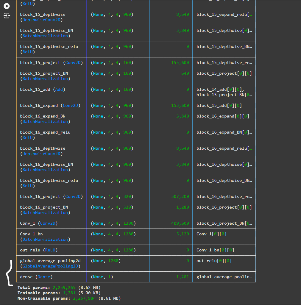
If we check the model summary, we can see GlobalAveragePooling layer and Prediction layer (dense) included

Compiling the Model

model.compile()

We have to provide optimizer, loss and metrics.

For optimizer, we use

tf.keras.optimizers.RMSprop(learning_rate=0.0001)instead of any string (If we specify optimizer with string, it will take all default value which we don’t want here)

we are using RMSprop as it’s MobileNet architecture and as it’s a pretrained model, we give a small learning rate (learning_rate=0.0001)

For loss, it’s binary_crossentropy as we are dealing 2 classes. Again the metrics will be accuracy as binary classification.

model.compile(optimizer=tf.keras.optimizers.RMSprop(learning_rate=0.0001), loss="binary_crossentropy", metrics=["accuracy"])

In the previous blogs, we performed all data set pre-processing steps manually from scaling to reshaping the dataset.

In this section, we haven't done any of these things except extracting the dataset. And now for the first time, we are going to use TensorFlow data generators to accomplish all of those data set pre-processing steps.

Since we are working with image data, we are going to use image data generator. And not only that, but we are going to create two generators, one for each data subset, one for our training data, and another one for validation.

Each Pre-trained model supports only specific input sizes. And if you want to use those models, we have to reshape our dataset to match some of those. In the case of MobileNet here, you can see all of supported input sizes ((96, 96), (128, 128), (160, 160), (192, 192), (224, 224))

And if we check the docstring, we will see that it accepts a lot of arguments and all of those arguments are used for pre-processing of image in some way.

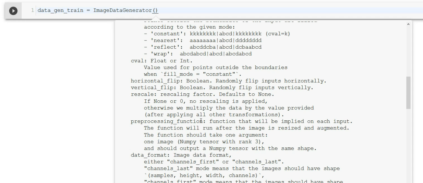
For our example, we are going to use only rescale, which is what we did so far.

data_gen_train = ImageDataGenerator(rescale=1/255.)

Divide each pixel by 255 to make them between 0 and 1.

We do it for train and validation both

data_gen_valid = ImageDataGenerator(rescale=1/255.)

The next step is to specify for each generator where to find the data set and how to preprocess it.

train_generator = data_gen_train.flow_from_directory()

To mean that we are taking the folder from directory.

Then we specify the folder , target size (same as our pixel shapes) , batch size and class_mode as binary to mean binary classification.

train_generator = data_gen_train.flow_from_directory(train_dir, target_size=(128,128), batch_size=128, class_mode="binary")

For validation dataset,

valid_generator = data_gen_valid.flow_from_directory(validation_dir, target_size=(128,128), batch_size=128, class_mode="binary")

Training the model

model.fit()

We will pass training data generator, train it for 5 times and validation data (valid_generator)

model.fit(train_generator, epochs=5, validation_data=valid_generator)

Evaluation

Now using validation generator, which we kept for evaluation, we check the evaluation

valid_loss, valid_accuracy = model.evaluate(valid_generator) # Use model.evaluate instead of model.evaluate_generator

print("Accuracy after transfer learning: {}".format(valid_accuracy))

Fine Tuning

- DO NOT use Fine tuning on the whole network; only a few top layers are enough. In most cases, they are more specialized.

In most cases, they are more specialized when CNN is trained. Lower layers are going to learn general features, lines, edges, corners and so on. But the top layers will get more abstract features about the data set as well.

For example, eyes, tails, ears and so on. And the goal of fine tuning is to adopt those specific parts of the network to our custom data set.

The goal of the Fine-tuning is to adopt that specific part of the network for our custom (new) dataset.

- Start with the fine tunning AFTER you have finished with transfer learning step. If we try to perform Fine tuning immediately, gradients will be much different between our custom head layer and a few unfrozen layers from the base model.

base_model.trainable = True

Here we have unfrozen layers

We have 154 layers in base model

print("Number of layersin the base model: {}".format(len(base_model.layers)))

Define a variable called fine tuned. And this will store an index of a starting layer from which point on we are going to fine tune. For this task.

Let's set this to 100. So we are going to fine tune all layers from 100 to 155.

fine_tune_at = 100

And to achieve this, if you remember, we unfroze the whole network. We need to freeze all layers before that.

for layer in base_model.layers[:fine_tune_at]:

layer.trainable = False

So, freezed all layers prior to layer 100.

Compiling for fine-tuning

Same as the compiling we did earlier

model.compile(optimizer=tf.keras.optimizers.RMSprop(lr=0.0001),

loss='binary_crossentropy',

metrics=['accuracy'])

Fine tuning

We have made some changes to our layers, right? Frozen some and unfreezed some.

Now, we will run the model and it will be finetuned

model.fit(train_generator,

epochs=5,

validation_data=valid_generator)

We have 100% accuracy on the training set and the worst accuracy on the validation dataset.

About 96%. The results indicate that our model overfitted.

In general, when you have a small dataset, it is not a good idea to perform the fine tuning step since it will overfit, which we have proven with this case as well.

We came very far by applying these techniques and we created a remarkable network that solved a binary classification with state of the art results.

Evaluating the fine tuned result

We have got a 96% accuracy with fine tuned model