Artificial Intelligence : Reinforcement Learning for Stock Market Trading (Part 41)
 Md Shahriyar Al Mustakim Mitul
Let’s apply RL for stock market trading
Install dependencies
!pip install tensorflow
!pip install pandas-datareader
import math
import random
import numpy as np
import pandas as pd
import tensorflow as tf
import matplotlib.pyplot as plt
import pandas_datareader as data_reader #to read trading data from tqdm import tqdm_notebook, tqdmfrom collections import deque #deque data structure

Let’s create an AI trader class
class AI_Trader():
def init(self, state_size, action_space=3, model_name=”Your desired name”)
Here, action_space will be Stay, Buy and Sell and thus, it’s 3
Model Building
  def model_builder(self):

    model = tf.keras.models.Sequential()

    model.add(tf.keras.layers.Dense(units=32, activation='relu', input_dim=self.state_size))

    model.add(tf.keras.layers.Dense(units=64, activation='relu'))

    model.add(tf.keras.layers.Dense(units=128, activation='relu'))

    model.add(tf.keras.layers.Dense(units=self.action_space, activation='linear'))

    model.compile(loss='mse', optimizer=tf.keras.optimizers.Adam(lr=0.001))

    return model
Trade function
  def trade(self, state):

    if random.random() <= self.epsilon:
      return random.randrange(self.action_space)

    actions = self.model.predict(state)
    return np.argmax(actions[0])
Our goal is to build a trade function that takes a state as an input and spills out an action to perform in the particular state. We are going to define it as death trade.
def trade(self, state):
For that state, we need to determine whether should we use an random generated action or should we use our model to perform that action?
Creating random action:
if random.random() <= self.epsilon: #depending on the epsilon value, we choose random action
return random.randrange(self.action_space) #return random action
Or else, we use our model to choose actions
#use model to choose an action
actions = self.model.predict(state) #we are going to use our NP dot argmax to return only an action which has the highest probability as the argument for the argmax.
Finally return an action with most probability
return np.argmax(actions[0]) #We will put actions of zero because of the output shape
To summarize:
It takes a state as an input and then generates a random number.
If that generated number is less than or equal to epsilon at the very beginning, it is going to be always less than epsilon.
This function will return totally randomly generated or chosen numbers between 0 or 2, and that is our actions. Then if this is not the case, this function will call our model and perform prediction based on the input state and return only the action that has the highest probability or the likelihood between those three actions.
Batch Trade
We will implement the last piece of the AI trader model. And that is the custom training function.
It will take a batch of saved data and train the model based on that. Let's define it.
def batch_train(self, batch_size):
And this function takes only one argument, and that is the batch size.
This argument could be anywhere from 32 to 256 or even more. And this is an additional hyper parameter that you want to play with.
We will always sample from the end of the memory, and this indexing method will help us to get exact number of points inside the batch of data.
for i in range(len(self.memory) - batch_size + 1, len(self.memory)):
Now that the for loop is done inside it called the batch list and append element from the memory itself.
batch.append(self.memory[i])
At this point, we have the batch of data and now it's time to iterate through it and to train the model for each sample from that batch
for state, action, reward, next_state, done in batch:
The order of variables is very important and inside the for loop right reward is equal to reward. Let's make sure that our agent is not in the terminal state. So let's write.
reward = reward
If not done. We are doing this very simple check to make sure that our agent is not in the terminal state and there are few more actions to be played.
if not done:
Based on this information alone, we can calculate a reward in a different ways. If the agent is in a terminal state, we will use the current reward as the reward. But if it's not in the terminal state and there are few more actions to be played, we are going to calculate the discounted total reward as the current reward. So in this if statement just right reward is equal to reward plus self dot gamma.
And you know the formula multiplied by p dot a max. And this function returns the maximum value from an input array. And that is exactly what we want. We want to return the highest value of predictions. And inside that function provide self dot model dot predict of next state and set that to zero because of the output size. And that is our discounted total reward.
reward = reward + self.gamma * np.amax(self.model.predict(next_state)[0])
After this, define the target variable which is predicted by the model as well.
target = self.model.predict(state)
At this point, it is just an action and we want to modify it with our current reward. And this is exactly why we use mean squared error instead of cross entropy loss.
Target of zero because of the output shape target[0], And then action.
target[0][action] = reward
And this is the action performed and that is all equal to reward. Now we have our target and our state.
Now it's time to fit the model.
self.model.fit(state, target, epochs=1, verbose=0)
For our target epochs.Just set to one because we will train the model very often on each sample from our batch. We don't want to print all of these training results, so just put verbose is equal to zero.
At the end of this function, let's decrease the epsilon parameter so we can stop performing random actions at one point.
if self.epsilon > self.epsilon_final:
self.epsilon *= self.epsilon_decay
Helper functions : Sigmoid function
One day the stock can be 200, but the next one it couldn't jump to 1000. The difference between them is the same as 45 to 200.
The difference as in the jump is the same. But the prices weren't. To handle this, we need to use sigmoid function to have the same number to represent this difference.
def sigmoid(x):
return 1 / (1 + math.exp(-x))
Helper functions : Price format
The next helper function is stock price format and that's the formatting function which will help us to print out the prices of the stock we bought or sold. It says if the number is negative. So we lost some money.
For example, it will add a minus in front of it. And we are using this string formatting to limit the printed number to only two decimal points. We are doing the same thing if the number is positive. Although we don't add the minus in front of it.
def stocks_price_format(n):
if n < 0:
return "- $ {0:2f}".format(abs(n))
else:
return "$ {0:2f}".format(abs(n))
Helper functions : Dataset Loader
We can visualize the data by
dataset = data_reader.DataReader(“AAPL”, data_source="yahoo")
To get Apple stock information, write AAPL as a string. The next argument that we have to specify is data source or which provider we should ask to provide that information for us.
In this case, we are saying data source is equal to Yahoo. And it's all what we have to provide.
After we finish with testing of this line, we are going to copy it and paste it right here in the function. But before we do that, let's check what it does. It will reach to Yahoo!
Get Apple stock information and save that to our dataset variable. Let's visualize it.
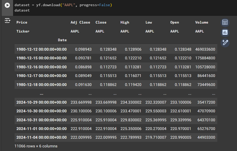
As you can see, it uses pandas. DataFrame object to store that information.
For each day we have some price of the stock. High Low is the highest and the lowest price for that day. Open is when a market is opened physically. For example, in New York. What was the price for that company? Then we have close. And close is a price similar to open one, but the price when the market is closed. Volume represents. How many stocks are there to be sold?
#We use the starting date (dataset.index[0]) and end date (dataset.index[-1])
start_date = str(dataset.index[0]).split()[0]
end_date = str(dataset.index[-1]).split()[0]
Working with the close column
close = dataset['Close'] #we are working with the Close value from the dataset
State Vector
we have to create a function that takes that data and generates states from it.
But before we start with the implementation of our state creator function, let's see how to transform the problem of stock market trading to a reinforcement learning setting. On this graph right here.
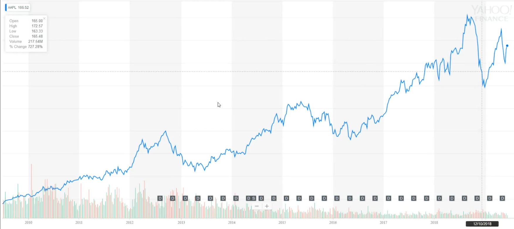
We have information about Apple stocks, prices from 2010 until today.
On the x axis. We have time information, but on the y axis we have prices of a stocks on a specific day, which is not visible right now on this graph.
This graph right here is taken from Yahoo Finance's, as you can see here.
And this blue main line on the graph shows how the value of a company changes over time.
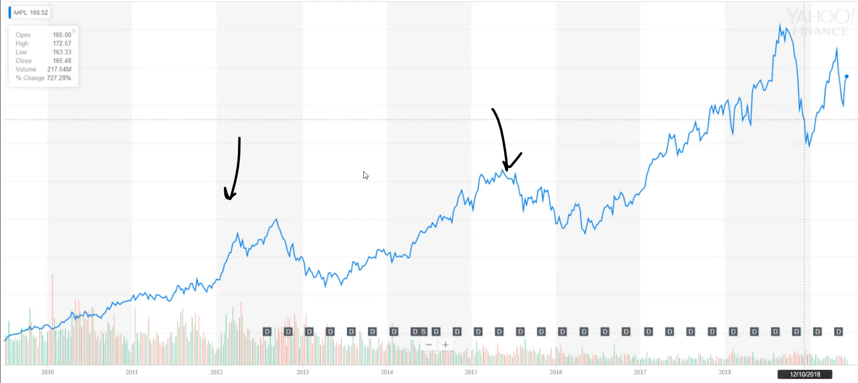
Let's see how to modify this data so reinforcement learning algorithm can understand it. Each point that is graph is nothing more but a floating number that represents a price of stocks on that day. Our task is to predict what is going to happen next. Is the price going down or going up?
And the next day. Based on that information, our agent will determine what to do sell, buy or stay and do nothing. Let's zoom at this part of the graph.
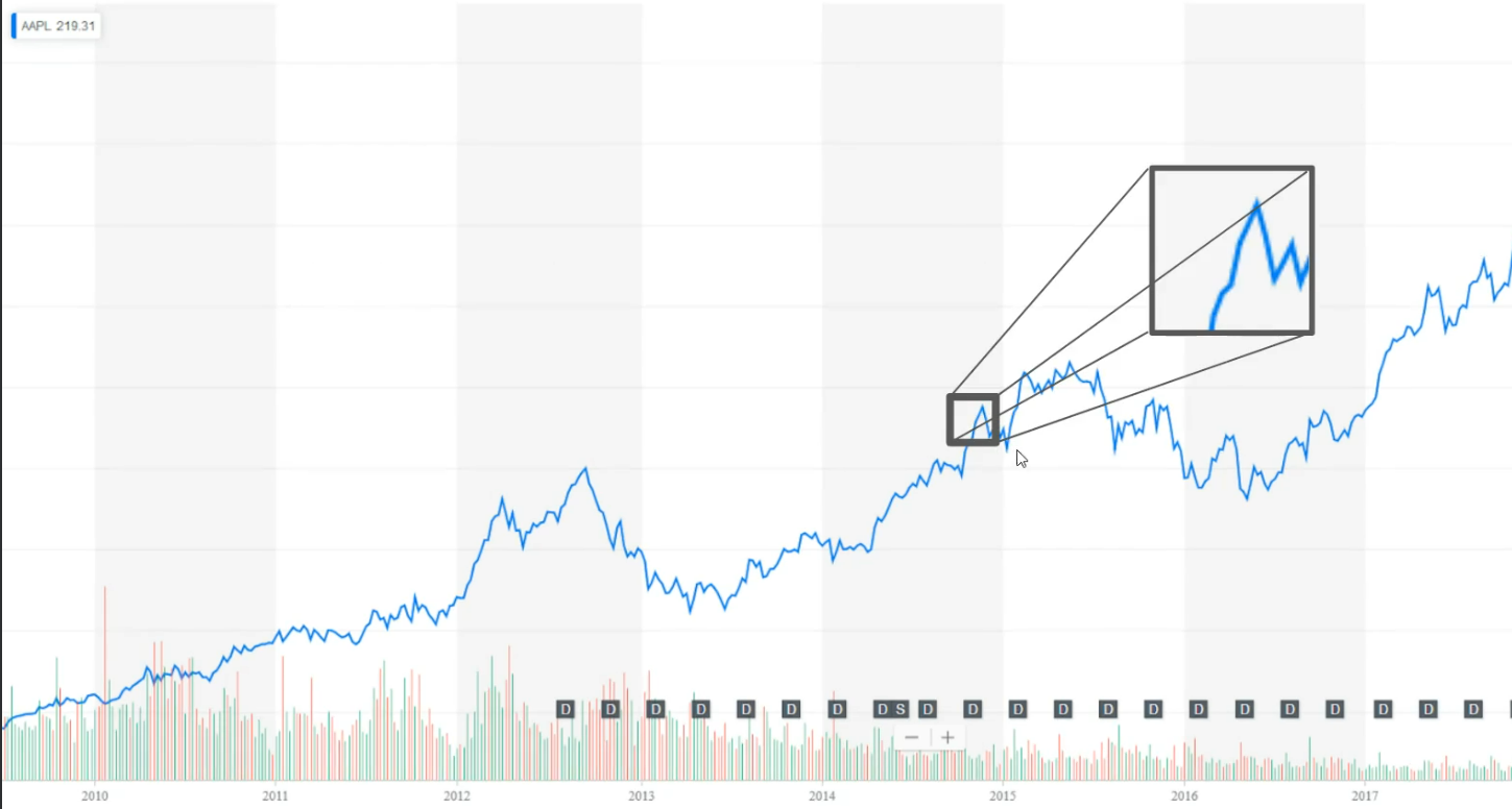
And as you can see here, we have information about six data points or six days, for example. Now, let's zoom even further and transform this part of the graph to numbers.
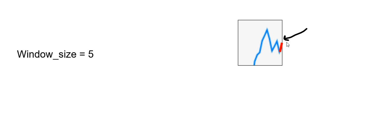
This red part right here is what we are trying to predict, and that is our target.Let's take this red line and transform it to number. And let's say it is 47.6 (Just randomly taken)
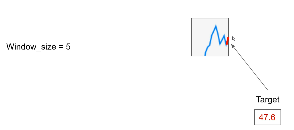
In this example right here, we have the window size of five, which is also the argument of the state creator function.
Based on this argument, we determine how many previous days we consider before predicting the current one.
And now we have our state made of five numbers where each number represents one day in the past. But based on this, it doesn't look right.
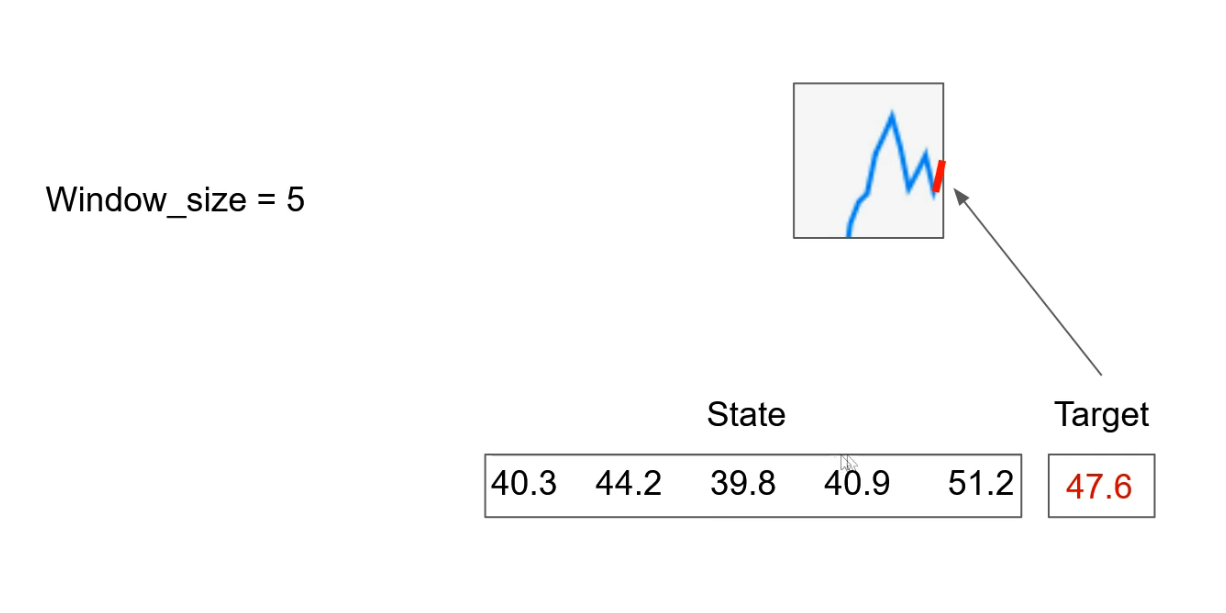
This is nothing more but a regression problem. We have some numbers and we are predicting our target, which is also a continuous number.
Now let's change our state to use differences between days as our state.
This information will represent price changes over time and potentially catch the trend in the future as well.
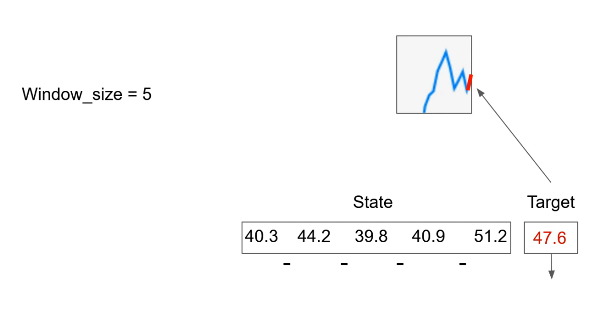
Now we have a state like this, and this new state has only four numbers and our window size was five. We will handle this in code.
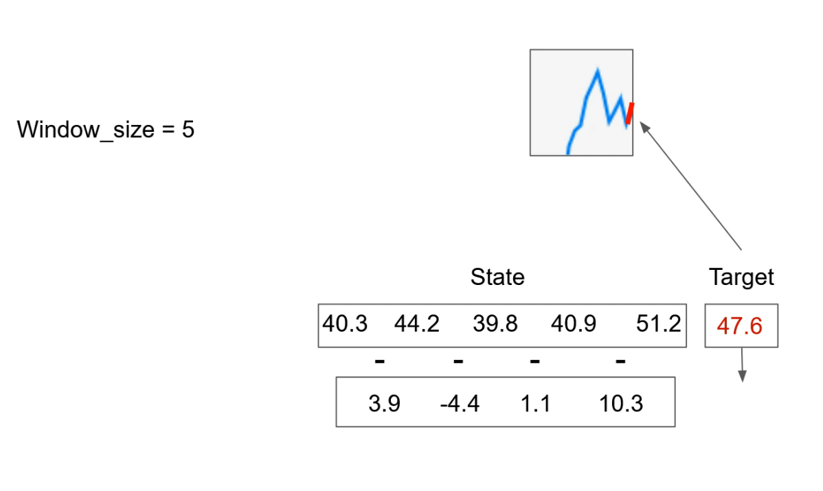
And now, because we have changed information over time, our action at the new state is “buy” because price was pretty high and we expect to drop again.
So based on that information, we are going to perform buy stocks at the new state and that's pretty much it.
Let's implement this strategy.
Here we have a function called state creator that takes three arguments data, which is the stock market data downloaded with the dataset loader function timestamp. This is the day in the dataset that we want to predict for It could be anywhere from zero to the length of data. And lastly, we have window size. This argument determines how many previous days we want to consider in our state to predict the current one.
def state_creator(data, timestep, window_size):
The first thing that we have to do is to calculate the starting ID.
So let's write. Starting ID is equal to.
starting_id = timestep - window_size + 1
And now we have to calculate the new starting day of our state. It is calculated like this. Timestep minus window size plus one.
For example, when the timestamp is zero or our agent is just starting and the window size is ten, the starting ID is minus nine.
This plus one is added because of the way we create our states. We don't want prices on certain days. But as we explained, differences between the current price and the previous price to see that change between days. And that's why we start with a plus one.
If starting ID is bigger than or equal to zero, this will handle the case when the starting ID is positive.
When we have that situation, we create state like this window of data is equal to data of starting ID until time. Step plus one.
if starting_id >= 0:
windowed_data = data[starting_id:timestep+1]
else:
windowed_data = - starting_id * [data[0]] + list(data[0:timestep+1])
If that is not the case and our starting ID is negative, we will append the first day info as many times as we need to match with the window size of a data window. Data is equal to then put minus in front of starting ID because starting ID at this point is negative. Then multiply it by then list of data of zero. This will replicate this member many times and now we need to append the rest of the elements to have the full window size of data.Plus then list of data from zero to timestamp plus one. Now we have our data from which we can create our state of data.
Let's define an empty list called state is equal to empty list. And after that we can iterate through the whole window of data list.
state = []
For I in range window size minus one. This minus one here because we have differences between the current element and the one after Wright state dot append and now we have to normalize the difference between the next day and the current day because prices can be very different.
for i in range(window_size - 1):
state.append(sigmoid(windowed_data[i+1] - windowed_data[i]))
We want to scale the difference between prices on the same scale so we have the same difference no matter the price. We are going to do that with sigmoid function. So let's write sigmoid of window data of I plus one minus window data of I. And now we completed the function that is going to create the state for us. The same state and the same method that we explained on the graph to complete the function, just the return a numpy array of the state.
Loading the dataset
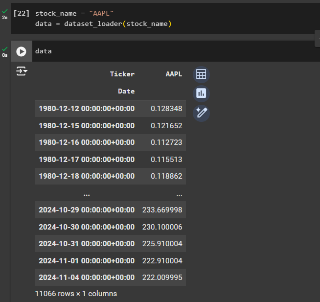
Using a dataloader, we can now load any specific stock information. For example, here we have loaded Apple stock (AAPL) using dataset_loader
We can check the AAPL dataset here
Training the AI trader
But now, before we proceed to the training loop, let's define the model and a few hyper parameters to use.
The first hyper parameter is the window size. Let's define window size is equal to ten. That means that we are going to use ten previous days to predict the current one.
In the previous sections, we used word epochs and in the reinforcement learning that is same as episode.
So we need to define how many times we are going to run through the whole data set or the whole environment. In this case, we will say episodes is equal to 1000. The algorithm is going to run very slowly. So we want wait for all of them to pass.
window_size = 10
episodes = 1000 batch_size = 32
data_samples = len(data) - 1
Then we'll specify 32 for the batch size.And in the end data samples is going to be equal to Len of data minus one. Since we are trying to predict the next day, we can't use the last one. So let's execute the cell and our hyper parameters are defined.
Trader model
Let's call it trader.
And that is going to be equal to our class trader. If you remember, it takes a lot of arguments, but since we define the action space to be free as default and the model name to be trader by default, we won't change that. So only thing that we have to specify is the state size and for us, that is our window size. Execute the cell and it is going to take some time to define the model.
trader = AI_Trader(window_size)
trader.model.summary()
Finally complete the training loop!
Check this code
Subscribe to my newsletter
Read articles from Md Shahriyar Al Mustakim Mitul directly inside your inbox. Subscribe to the newsletter, and don't miss out.
Written by
