Using Lasso Model to Predict Chess game Outcome in R
 Adeniran Emmanuel
Table of contents

Origin of Chess Game
The Ancient Roots
The longest recorded chess game lasted 269 moves and took 20 hours and 15 minutes to complete.
The origins of chess can be traced back to ancient India, around the 6th century AD. It evolved from a game called Chaturanga, which translates to "four divisions" - a reference to the four components of the Indian military: infantry, cavalry, elephants, and chariots. These components were represented by the pawn, knight, bishop, and rook, respectively.
Over centuries, Chaturanga spread to Persia, where it transformed into Shatranj. The game further evolved as it traveled through the Arab world and eventually reached Europe in the 10th century. The modern rules of chess, including the queen's increased power, emerged during the 15th century.
The Art of Opening (Opening_eco)
The opening phase of a chess game is crucial, as it sets the stage for the middle game and endgame. Chess players spend countless hours studying and practicing various openings, seeking to gain an advantage over their opponents.
An opening is a sequence of moves played at the beginning of a chess game. There are numerous openings, each with its own distinct characteristics and strategies. Some of the most popular openings include:
The Ruy Lopez C60: A classic opening characterized by the moves e4 e5 Nf3 Nc6 Bb5.
The Sicilian Defense B20: A sharp and tactical opening, often leading to complex and dynamic positions.
The Queen's Gambit D06: The Queen’s Gambit is the most popular chess opening starting with 1.d4. It begins with the moves 1.d4 d5 2.c4..
The King's Indian Defense E60: Looking for a proven and sound way to play for the win against the Queen’s Gambit from move 1? Then the King's Indian Defense (1.d4 Nf6 2.c4 g6) is the chess opening you are looking for
By understanding the nuances of different openings, players can gain a significant advantage in the early stages of the game. However, it's important to remember that opening theory is just one aspect of chess. Tactical skill, strategic thinking, and positional understanding are equally important for success.
The current world chess champion is a computer program called Stockfish. It can calculate billions of positions per second.
What is Lasso Regression?
Lasso regression is a type of linear regression model that include a regularization technique called L1 regularization. This technique adds a penalty term to the loss function, which encourages the model to shrink the coefficients of less important features towards zero. As a result, Lasso regression can perform feature selection automatically and prevent overfitting especially when dealing with high dimensional dataset.The regression cannot handle categorical and non-numeric variables as our independent variable so we convert the categorical data to dummy variables.
To use the Lasso Regression in R, we make use of the multinom_reg() function in the tidymodels package and specify our model parameters.The parameter “mixture = 1” specify that we want to use Lasso Regression from the function and also we would tune the penalty because of the hyperparameter.
Further explaination would be made about how to tune Lasso Model in the Case Study
Lasso Regression model can be used for both regression and classification problems
We can use the multinom_reg() function to compute the Lasso regression model when the mixture = 1
```{r Model Specification}
library(tidymodels)
chess_mod <-
  multinom_reg(penalty = tune(),
             mixture = 1) |>
  set_engine("glmnet") |>
  set_mode("classification")

chess_mod
```
Advantages of Lasso Regression Model
Feature Selection
Lasso regression identifies and select the most relevant features from a large pool of potential predictors and is easier to interprete and less prone to overfitting
Interpretability
Lasso models often result in sparse solutions and this makes it easier to understand the underlying relationship between the feature and the target variable
Handling High-Dimensional Data
Lasso regression can handle large datasets with a large number of features, even when the number of features exceeds the number of observations. Lasso model also reduces the computational cost of model training and Prediction
Regularization
The L1 Regularization helps to prevent overfitting by shrinking the coefficient of less important features towards 0.
Metrics of Evaluating the Lasso Regression Model
There are various metrics to evaluate the Lasso Regression Model when we have to solve a regression model such as MAE,RSQUARED,MSE, e.t.c. and when used for classification problems have some merics we use to evaluate the model such as Accuracy,Brier_class,ROC_AUC, e.t.c.
We would focus on three metrics we use to evaluate the model in R to better understand the case study at the end of this article
Brier class
While the Brier score is primarily used for probabilistic predictions, especially in binary classification, it can be adapted to evaluate the performance of Lasso regression models, particularly when the target variable is binary
The Brier score measures the mean squared difference between the predicted probability and the actual outcome (0 or 1).
A lower Brier score indicates better model performance
ROC-AUC
While Lasso regression is primarily a regression technique, it can be adapted for binary classification by setting a threshold on the predicted probabilities. Once you have probability predictions, you can calculate the ROC-AUC to evaluate the model's performance.
Mean Squared Error (MSE)
MSE is a common metric used to evaluate the performance of regression models, including Lasso regression. It measures the average squared difference between the predicted and actual values. A lower MSE indicates a better-fitting model.
What is Weighted Log Odds
Odds are simply a way to express the probability of an event occurring.
Odds are a way to express the probability of an event occurring. They represent the ratio of the probability of the event happening to the probability of it not happening.
For example:
If the odds of an event are 3 to 1, it means that the event is 3 times more likely to happen than not happen.
If the odds are 1 to 2, it means the event is 2 times more likely not to happen than to happen.
While odds and probability are related, they are not the same.
Odds vs. Probability:
While odds and probability are related, they are not the same. Probability is a number between 0 and 1, representing the likelihood of an event. Odds, on the other hand, are a ratio of probabilities.
Log odds is simply taking the log of the event occuring or not occuring.
library(tidylo)
chess |>
  count(opening_eco,winner) |>
  bind_log_odds(winner, opening_eco,n)
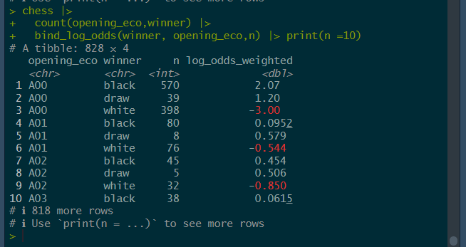
Interpretation of the result of bind_log_odds()
We can also Plot the Graph of the top opening_eco that has the biggest odds for the occurence of the winning event
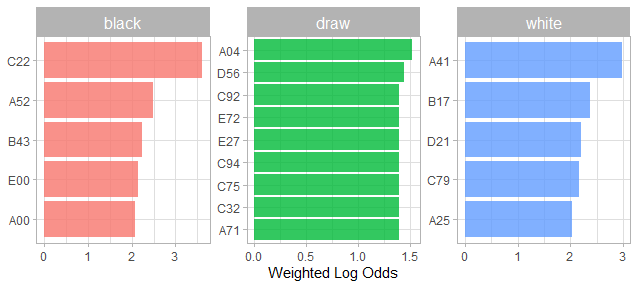
Interpretation of the Plot
Case Study - A Lasso Regression Model to Predict the Outcome of a Chess Game
About the Data
This Data is gotten from Lichess from Kaggle and it has over 20,000 games collected from a selection of users on the site Lichess.org with the following variables
Game ID;
Rated (T/F);
Start Time;
End Time;
Number of Turns;
Game Status;
Winner;
Time Increment;
White Player ID;
White Player Rating;
Black Player ID;
Black Player Rating;
All Moves in Standard Chess Notation;
Opening Eco (Standardised Code for any given opening, list here);
Opening Name;
Opening Ply (Number of moves in the opening phase)
Now Lets Draw Some Insight from the Dataset using R
#Loading Necessary Libraries
library(tidyverse)
library(tidylo)
library(tidytext)
library(tidymodels)
library(textrecipes)
library(glmnet)

#Reading in the Dataset
chess <- read_csv("Chess Project/chess.csv")

chess

Let’s go do some Exploratory Data Analysis
#Does the Player Rating affect the outcome of  the game?
chess |>
  select(white_rating,black_rating,winner) |>
  pivot_longer(-winner) |>
  ggplot(aes(value,fill = name)) +
  geom_histogram(alpha = 0.6, position = "identity") +
  facet_wrap(vars(winner)) +
  labs(
    x = "Ratings",
    y = "Count",
    fill = NULL
  )
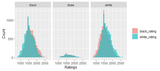
Winner Outcome and Players Ratings
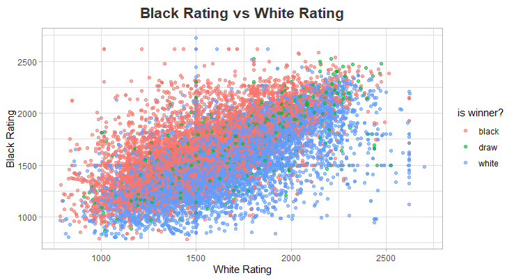
Does the Player rating not really affect the Outcome of the game?
chess |>
  ggplot(aes(white_rating,black_rating, color = winner)) +
  geom_point(alpha = 0.6) +
  labs(
    title = "Black Rating vs White Rating",
    color = "is winner?",
    y = "Black Rating",
    x = "White Rating"
  ) +
  theme(
    plot.title = element_text(
      hjust = 0.5,
      size = 16,
      face = "bold",
      color = "gray20"
    )
  )
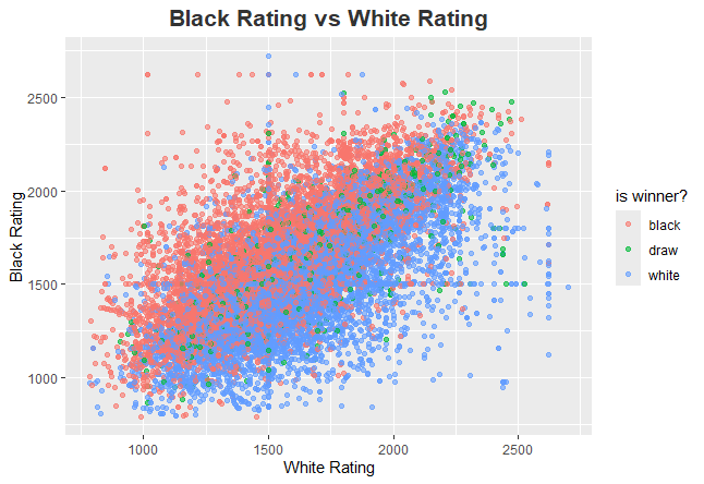
Black Rating vs White Rating Plot Interpretation
Now Let’s Look at the log odds and how it can help us understand out data more accutately and see which opening eco decided the outcome of the game
library(tidylo)
chess |>
  count(opening_eco,winner) |>
  bind_log_odds(winner, opening_eco,n)

Weighted Log Odds Interpretation
Now let’s take the top 15 opening ecos and see how they affected the outcome
library(tidylo)
chess |>
  count(opening_eco,winner) |>
  bind_log_odds(winner, opening_eco,n) |>
  group_by(winner) |>
  slice_max(log_odds_weighted, n = 5) |>
  ggplot(aes(log_odds_weighted,fct_reorder(opening_eco,log_odds_weighted),fill = winner)) +
  geom_col(show.legend = FALSE) +
  facet_wrap(vars(winner),scales = "free") +
  labs(
    x = "Weighted Log Odds",
    y = NULL
  )

Weighted Log Odds Plot Interpretation
Lets Proceed to Modeling our Data using Lasso Regression for Classification
# Wespend our data budget here by splitting our data into testing and trainins sets
set.seed(123)
index <- chess |>
  mutate(victory_status = as_factor(victory_status),
         wwinner = as_factor(winner)) |>
  initial_split(strata = winner)

chess_train <- training(index)
chess_test <- testing(index)
#Creating some Resampling Folds for Validation
set.seed(234)

chess_folds <- vfold_cv(chess_train, strata = winner)

chess_folds
#Create a Recipe for the Data Preprocessing
chess_rec <-
  recipe(winner ~  victory_status + white_rating + black_rating + opening_eco + opening_name + moves, data = chess_train) |>
  update_role(opening_name, new_role = "id") |>
  step_normalize(all_numeric()) |>
  step_tokenize(moves) |> # To split out moves into separate observations
  step_tokenfilter(moves, max_tokens = 100) |>
  step_tfidf(moves) |>
  step_dummy(all_nominal_predictors())


chess_rec |> prep() |> bake(new_data = NULL)
#Create the lasso Regression Model with "mixture = 1"
chess_mod <-
  multinom_reg(penalty = tune(),
               mixture = 1) |>
  set_engine("glmnet") |>
  set_mode("classification")

chess_mod
#Create a grid to select possible values of the penalty regularization
chess_grid <-
  grid_regular(penalty(range = c(-5,0)), levels = 20)

chess_grid
#Put the recipe and the model into a Workflow object for better documentation
chess_wf <- workflow(chess_rec,chess_mod)

chess_wf
#Create the model by using the tune_grid() function
doParallel::registerDoParallel()
set.seed(345)

chess_res <-
  tune_grid(
    chess_wf,
    chess_folds,
    chess_grid
  )

chess_res
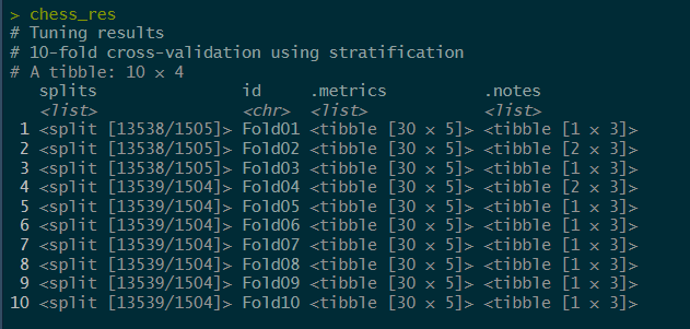
We have now fitted our Model with the training set resample folds and we can observe the metrics before fitting it finally with our training set and evaluating it on our testing set
autoplot(chess_res)
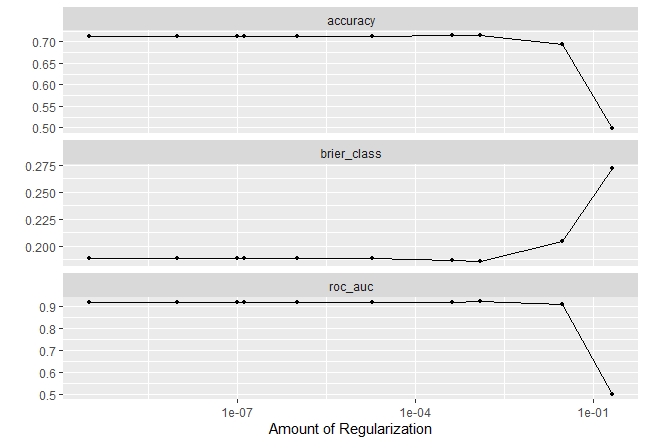
Summary of the Model Performance Plot
Lets check for the penalty term with the best performance and fit it finally
chess_final <-
  chess_res |>
  select_by_one_std_err(metric = "roc_auc",
                        desc(penalty))

chess_final

Penalty Value for the final model
#Finalize the workflow with the penalty term and last_fit it
final_res <-
  chess_wf |>
  finalize_workflow(chess_final) |>
  last_fit(index)

final_res

#we can check for the important variables in our model
library(vip)
extract_workflow(final_res) |>
  extract_fit_parsnip() |>
  vip(aestheticcs = list(fill = "midnightblue")
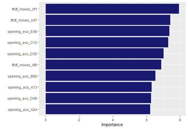

Final Result Interpretation
Lets take a look at the confusion matrix and see how well our model was able to predict the outcome
#Print out the confusion matrix
collect_predictions(final_res) |>
  conf_mat(winner,.pred_class)

#Plot the confusion matrix using autoplot()
collect_predictions(final_res) |>
  conf_mat(winner,.pred_class) |>
  autoplot()
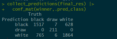
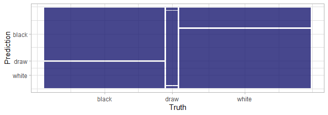
Interpreting the confusion Matrix
Lastly lets take a look at the ROC_AUC
collect_predictions(final_res) |>
  roc_curve(winner,.pred_black:.pred_white) |>
  ggplot(aes(1-specificity,sensitivity,
             color = .level)) +
  geom_abline(slope = 1,color = "gray50",
              lty = 2, alpha = 0.7) +
  geom_path(size = 1.5,alpha = 0.8) +
  labs(
    color = NULL
  ) +
  coord_fixed()
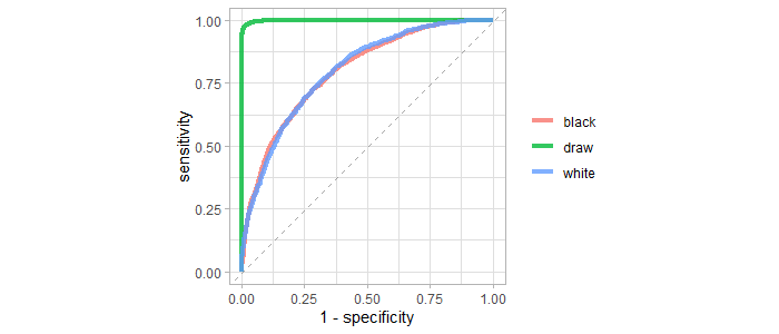
ROC_AUC Plot Interpretation
Yes We did It!.
You can access the code here on my github accountand also follow me on linkedin for more R tips
Follow me:
Adeniranbanjo07@gmail.com
Subscribe to my newsletter
Read articles from Adeniran Emmanuel directly inside your inbox. Subscribe to the newsletter, and don't miss out.
Written by
