Binary Variable Average Evaluation Methods

TL;DR

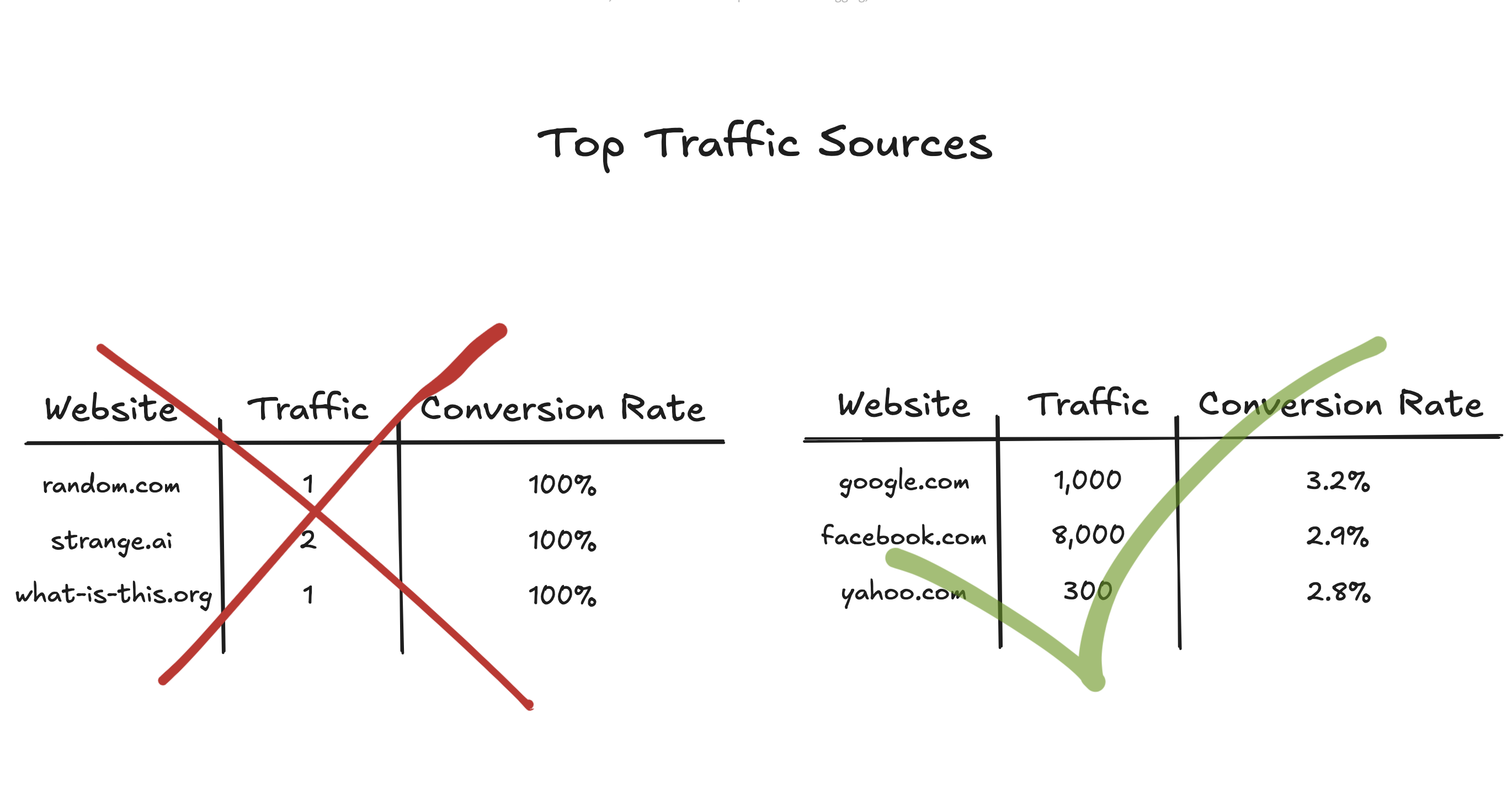
Some metrics are an average of the binary variable (0/1, False/True) — conversion rate, churn rate, etc. These metrics might not represent the actual value when there is a small sample size beneath them (one web session with one conversion leads to a 100% conversion rate). In this blog post, I describe several ways to tackle this issue with fully reproducible code.

Problem statement

Let's talk about binomial proportion measures and two ways of reasonably calculating them. Essentially, these measures are percentages derived from binary variables (0, 1). For instance, conversion rate is a proportion measure that is calculated as an average from the binary variable is_transaction, another example is click-through rate — it is an average from is_click. We can go on with examples: churn rate, order fulfillment rate, delivery rate, and cart abandonment rate, all of which fall into this category. Another less straightforward example is a rating score (thumb ups and downs), we can encode positive and negative reactions as zeros and ones so that the average of this encoding will be % of how people like something.

The issue occurs when we don't have enough data to evaluate the actual proportion correctly. One example is sorting. If you sort landing pages by conversion rate you might end up having landing pages with a 100% conversion rate on the top, simply because they just had one session and by luck, it was a converted session. Another use case is when you are going to use a proportion measure in some downstream calculations, for example, if you are building a predictor model where this percentage measure is a feature. Weak evaluation can significantly reduce the importance of such a feature.

For visibility, let’s use the data of an e-commerce shop that has traffic from various marketing sources. We want to see the top-performing sources by conversion rate (CVR). For these purposes, let’s take Google Analytics data from the BigQuery public dataset (available here, details on how to use it for free are here). It contains web data for 12 months (August 2016 to August 2017) of obfuscated Google Analytics 360 data from the Google Merchandise Store, a real e-commerce store that sells Google-branded merchandise.

Firstly, let’s take a look at what we will see if we simply sort traffic sources by CVR.

WITH data AS (
  SELECT 
    trafficSource.source AS traffic_source,
    SUM(totals.visits) AS visits,
    COALESCE(SUM(totals.transactions), 0) AS conversions,
    (COALESCE(SUM(totals.transactions), 0) / SUM(totals.visits)) AS CVR
  FROM `bigquery-public-data.google_analytics_sample.ga_sessions_*`
  GROUP BY trafficSource.source
)

SELECT 
  traffic_source AS `Traffic Source`,
  visits AS Visits,
  conversions AS Conversions,
  ROUND(CVR * 100, 2) AS CVR
FROM data
ORDER BY CVR DESC

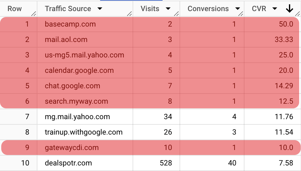
We can see that it’s not very informative because in the top-10 sources by CVR, there is only one decent channel (and potentially two good enough ones), whereas all the rest simply don’t have enough traffic, but were lucky to get some conversions. It’s quite distractive to go through this sorted list.

Solution 1: Interval

The first solution to the problem is to use the lower bound of the confidence interval. In this way, sources with a small amount of traffic will have quite a low lower bound estimate, whereas sources with a lot of traffic will have a lower bound close to the calculated value.

There are plenty of ways to calculate the lower bound for the binomial proportion metric (check out this for the list of them). As many researches show, the Wilson score is considered to be the most accurate and robust. So it’s a no-brainer which one to choose if you don’t have any specific requirements. For our case when we want to have a relevant estimation of the small sample sizes it is beneficial to add the continuity correction, which will provide a wider confidence interval.

The formula is the following:

$$w^-_{cc} = \frac{1}{1 + \frac{z^2_{\alpha}}{n}}\Bigg(\hat{p}_{cc} + \frac{z^2_{\alpha}}{2\ n}-\frac{z_{\alpha}}{2\ n}\sqrt{ 2\ n\ \hat{p}_{cc}\ (1-\hat{p}_{cc}) + z^2_{\alpha}}\Bigg)$$

Where:

$w$ — stands for Wilson's confidence interval

$-$ (in $w^-$) — means lower bound (as we are not interested in the upper bound for our task)

$cc$ — stands for continuity correction

$z_{\alpha}$ — is a z-score that depends on the accepted error $\alpha$. For the confidence level 95% $\alpha = 1 - 0.95 = 0.05$, and $z_{0.05} = 1.96$

$n$ — is a number of samples

$\hat{p}$ — is our proportion

$\hat{p}_{cc}$ — is the proportion with the continuity correction that has the following formula $\hat{p}_{cc} = max\{\hat{p} - \frac{1}{2\ n},\ 0\}$

The SQL calculation of it is straightforward, although a bit bulky:

(1 / (1 + 3.8416 / n)) *
(
    GREATEST(p - 1 / (2 * n), 0) +
    3.8416 / (2 * n) -
    1.96 / (2 * n) *
    SQRT(
      2 *
      n *
      GREATEST(p - 1 / (2 * n), 0) *
      (1 - GREATEST(p - 1 / (2 * n), 0)) +
      3.8416
    )
)

We can wrap it up into a dbt macro:

{% macro wilson_lower_bound(p, n) %}

    {% set z = 1.96 %}
    {% set z_2 %}
    POW({{ z }}, 2)
    {% endset %}
    {% set p_cc %}
    GREATEST({{ p }} - 1 / (2 * {{ n }}), 0)
    {% endset %}

    1 / (1 + {{ z_2 }} / {{ n }}) *
    (
        {{ p_cc }} +
        {{ z_2 }} / (2 * {{ n }}) -
        {{ z }} / (2 * {{ n }}) *
        SQRT(
            2 *
            {{ n }} *
            {{ p_cc }} *
            (1 - {{ p_cc }}) +
            {{ z_2 }}
        )
    )

{% endmacro %}

The usage of the macro is as straightforward as this:

WITH data AS (
  ...
)

SELECT 
  ...
  ROUND(({{
    wilson_lower_bound('CVR', 'visits')
  }}) * 100, 2) AS `CVR Lower CI`
FROM data
ORDER BY `CVR Lower CI` DESC

If we apply this to our web data, we will have the following result:

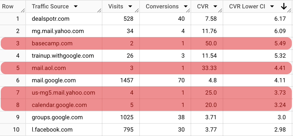
As we can see, it is much better than initial sorting. But there is still a problem, the channels with few sessions can be still very high in the sorted list. We can tackle by adjusting the Z-score (increasing the confidence level to 99%). Alternatively, we can use the next solution.

Solution 2: Bayesian approach (beta)

Another approach is to use Bayesian inference. An average of i.i.d. binomial variables has a beta distribution. When we perform Bayesian inference we deal with prior (our prior assumptions regarding the metric) and posterior (our final estimation of metric based on prior assumptions and new data) distributions. Beta distribution $Beta(\alpha,\ \beta)$ has only two parameters: $\alpha$ — a number of positive samples (or ones), and $\beta$ — a number of negative samples (or zeros). The handy feature is that if a prior assumption has a beta distribution, the posterior has also a beta distribution $Beta(\alpha + \alpha_{data},\ \beta + \beta_{data})$, where $\alpha_{data}$ and $\beta_{data}$ are the newly gathered data for positive and negative samples respectively. What we are interested in is the average of these variables (in our example — CVR). An average of the beta distribution is $\frac{\alpha}{\alpha + \beta}$. It means that we can simply set some prior distribution through $\alpha$ and $\beta$, then calculate the metric with Bayesian correction $\frac{\alpha + \alpha_{data}}{\alpha + \beta + \alpha_{data} + \beta_{data}}$.

How does it work? When we don’t have enough data, our average estimation will lean toward the prior assumption. However, once we have enough data, our prior assumption will not weigh as much as fresh data.

The question is how to set the prior values for $\alpha$ and $\beta$? One way is by defining the prior mean and variance for our variable. Then we will only need to solve the following system of equations:

$$\begin{cases} E[X] \equiv \mu = \frac{\alpha}{\alpha + \beta}\\ var[X] \equiv \sigma^2 = \frac{\alpha\ \beta}{(\alpha + \beta)^2\ (\alpha + \beta + 1)} \end{cases}$$

This leads us to the following equations:

$$\displaylines{\alpha = \mu\ \Bigg(\frac{\mu\ (1 - \mu)}{\sigma^2} - 1 \Bigg)\\ \beta = (1 - \mu)\Bigg( \frac{\mu(1 - \mu)}{\sigma^2} - 1 \Bigg)}$$

From the practical perspective it is quite easy to define the prior mean, coming back to our example with conversion rates we can use one of the following (but not limited to):

Historical conversion rate for our website
Historical conversion rate for each group of traffic sources (marketing channels)
Industry benchmark conversion rate

Much less straightforward is how to define the variance (confidence in our prior mean). One way is to set a reasonable range of values (saying that the conversion rate cannot be less than 0% and more than 4%). Then, using the two-sigma rule we can evaluate the standard deviation, which is the square root of variance. In other words, we will be saying that we are 95% certain that our metric lies in the selected range. Note, that this is a simplification, because we deal with beta distribution, which is asymmetrical, and the two-sigma rule is applied to the symmetrical normal distribution. But it does not hurt much to use this rule for practical purposes. Let’s say our prior mean for conversion rate is 1% ($\mu = 0.01$), and the reasonable range is from 0% to 4%. We are saying that 4% is lying in 2 sigmas from 1%, or in other words $2\sigma = 0.04 - 0.01 = 0.03$. That means that $\sigma = 0.015$, and variance $\sigma^2 = 0.000225$.

If we apply these values to the formulas of $\alpha$ and $\beta$ above, we will have our prior distribution $Beta(0.4,\ 42.6)$. Now the most interesting part is that for a traffic source with only one session that led to conversion (so the conversion rate is 100%), our posterior distribution will be $Beta(1.4, 43.6)$, and the posterior conversion rate will be only 3.1% ($\frac{1.4}{1.4 + 43.6} = 0.031$). As we have promising data of a 100% conversion rate, we hope that this source might have above the average conversion rate, but only to some conservative degree.

SELECT 
  ...
  ROUND(
    ((0.4 + conversions) / (0.4 + conversions + 42.6 + visits)) * 100,
  2) AS `CVR Beta`
FROM data
ORDER BY `CVR Beta` DESC

Let’s take a look at how the results table will look with such an approach:

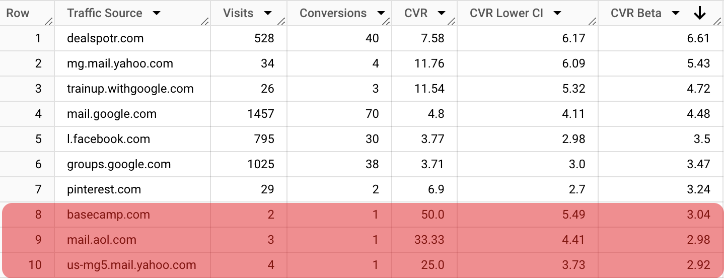
We can see that the basecamp source went from the 3rd place to the 8th. This is an improvement because, from a practical standpoint, it is risky to draw a solid conclusion from two observations.

Currently, we are not comparing apples to apples, because the lower 95% confidence interval means we are 95% certain the actual value is no lower than the calculated value. Whereas the mean of Beta distribution means the expected value. To make the comparison more reasonable it is better to calculate the 2.5 percentile of the Beta distribution (95% confidence interval). Luckily, with the Bayesian approach our result is not a single value, but the whole distribution, thus we can calculate percentile using percentile point function (PPF). It is challenging to calculate it with plain SQL, but still possible using user-defined functions, or dbt Python models. In Python, it is as simple as that:

from scipy.stats import beta
beta.ppf(0.025, 0.4 + conversions, 42.6 + visits)

The result is:

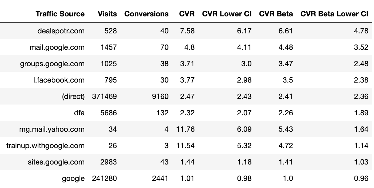
There are no more low-volume websites in the top-10 traffic sources, which means our sorting is much more reliable now.

If you want to be more scientifically backed, you can replace the two-sigma approach with 95% interval estimation using beta distribution cumulative distribution function (CDF) and solving an optimization problem. I will not dive into it, but will provide the code and mention that the results in our setting turn out to be very similar: $Beta(0.4, 43.7)$

import scipy.special as sp
import scipy.optimize as opt

confidence = 0.95
upper_value = 0.04
mean_value = 0.01
alpha_initial_guess = 1.0

def objective(alpha):
    beta = alpha * (1 - mean_value) / mean_value
    cdf = sp.betainc(alpha, beta, upper_value)
    return (cdf - confidence) ** 2

result = opt.minimize(objective, alpha_initial_guess, bounds=[(0.1, 100)])
alpha_estimated = result.x[0]
beta_estimated = alpha_estimated * (1 - mean_value) / mean_value

print(f"Estimated alpha: {alpha_estimated}")
print(f"Estimated beta: {beta_estimated}")

Conclusion

In this blog post, I went through several approaches to calculate robust binary variable averages. Most of them are possible to use in plain SQL, which is quite convenient. These calculations are very useful for dashboards or machine learning models. Below, you can find code with fully reproducible example and relevant links.

In the further posts, I am going to cover robust calculations for other types of variables. Stay tuned.

Robust evaluation of binary variable average

Table of contents

Problem statement

Solution 1: Interval

Solution 2: Bayesian approach (beta)

Conclusion

Links to code and other materials

Subscribe to my newsletter

Kliment Merzlyakov

Kliment Merzlyakov