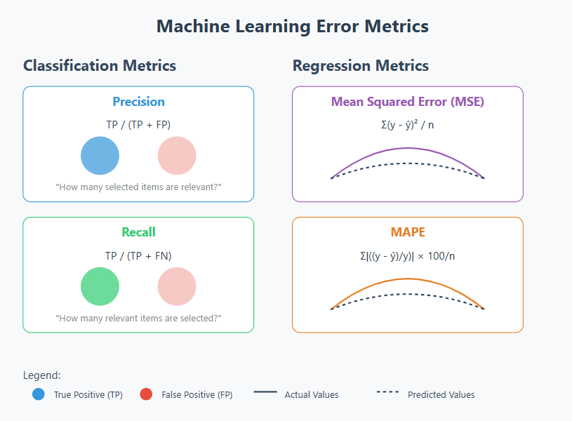
Hi there, in this post, I will discuss the metrics that are used to evaluate how accurate machine learning models are. I hope that helps. You can use this page as a cheat sheet.

At its core, what we all do when deriving a machine learning model is make a hypothesis. We are adding the features that we think have the most impact on the model; there is a hypothesis here. To explain with a very simple example, we have information such as the final letter grades students receive in courses, the time they spend on the course, and their homework submission rates. We take those that we really think affect the course grades and put them into a linear regression model, and when predicting pass or fail, we use a logistic regression model. Here, our claim that these features have an impact is a hypothesis; and the accuracy of hypotheses is measured by values such as sensitivity, specificity, F1 score, and p-value; therefore, those working in academia or in the field of statistics are familiar with these concepts.

Let's assume, as a classic example, that you are being tested for a disease.

True positive: You think you have the disease (you predicted the test would be positive) and the test came back positive. So you thought the hypothesis you proposed was correct, and it turned out to be correct.

False positive: You think you have a disease (your guess is positive), but the test you took came back negative.

False negative: You think you don't have the disease (your guess is negative), but you took a test and it came out positive.

True negative: You think you don't have the disease (your prediction is negative), you took the test, and it came out negative.

Let's give another example. You are predicting whether Team A will win an upcoming basketball game, and you have made a null hypothesis about Team A’s chances.

• True positive: You thought Team A would win, and they did.

• True negative: You said Team A would lose, and they lost.

• False positive: You said Team A would win, but they lost.

• False negative: You thought Team A would lose, but they won.

If you get too carried away and place bets, you might make type I and type II errors, which are well-known in statistics. Here, the null hypothesis (the situation you believe will occur, your assumption, null hypothesis) is that you think Team A will win.

• Type I error: You bet on Team A to win, but they lost. (False Positive)

• Type II error: You thought Team A would lose; bet on it, but they won. (False Negative)

Confusion Matrix

The confusion matrix allows us to organize the data I mentioned above and perform calculations on it. It would be better to explain the complexity matrix through the matrix itself.

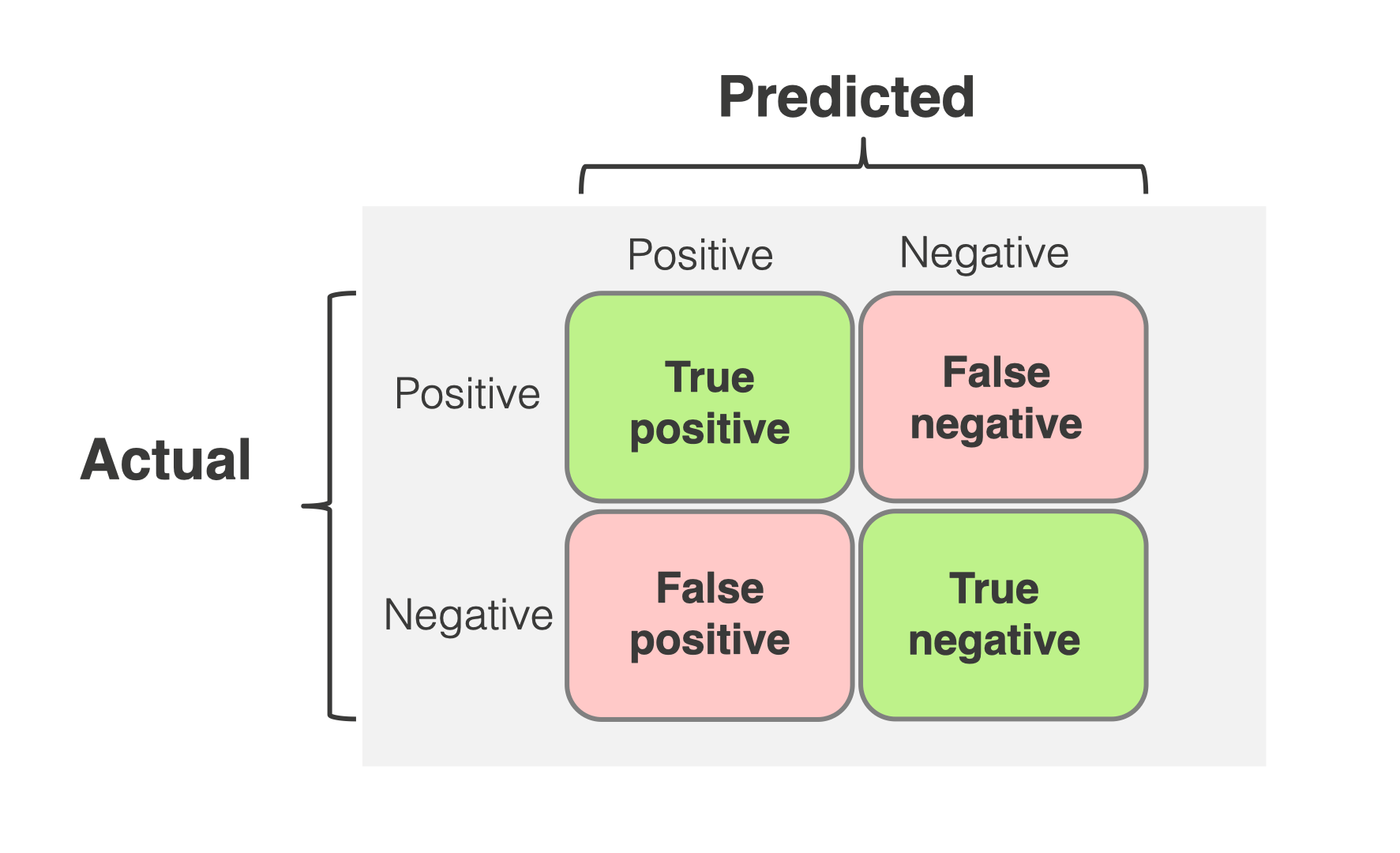
In the confusion matrix, the rows contain the counts of predicted positives and negatives, while the columns contain the counts of actual positives and negatives. The confusion matrix is used not only for dichotomous data like positive and negative, but this is outside the scope of our topic right now. If you're curious, you can see one at the end of the article.

Let's give another example using a disease: You want to test for a disease with a one in a hundred thousand chance of contracting it, and the test promises you 99.999% accuracy. Would you take this test? Do you think accuracy is a sufficient metric here?

The main issue here is that in this classification (sick/not sick) problem, most of the data belongs to the not sick class, meaning one class is overshadowing the other. In such cases, we refer to metrics like recall and precision.

Recall

Let’s take a very simple example to understand Recall. In a school attendance system, true positives are students marked present who are actually in class, and false negatives are students marked absent who are actually in class. We focus on recall because of false negatives in the denominator—students incorrectly marked absent when they're actually present. For a teacher, marking a student absent when they're actually present is a serious error since it could affect their attendance record and grades.

Following this logic, if you mark everyone present, the recall will be 1, but this isn't ideal. That's why we don't set fixed recall targets. Instead, for each attendance tracking system, we determine appropriate recall and precision values based on how many false absences we can tolerate. The True Positive Rate and Sensitivity we use in the ROC curve are technically the same as recall.

Formula:

Example:

• 40 students are actually present in class

• System correctly marks 35 as present (True Positives)

• The system incorrectly marks 5 present students as absent (False Negatives)

• Recall = 35 / (35 + 5) = 0.875 or 87.5%

Precision

Precision is a metric in predictive analysis that measures the accuracy of positive predictions. It represents the proportion of true positive results out of all positive predictions made by a model.

Precision in the attendance system refers to the percentage of students who are actually present out of those who are marked as present. In the denominator, precision examines false positives, or students who are marked present but are absent. Marking an absent student as present is a challenge for teachers since it may conceal attendance problems.

According to this reasoning, marking everyone absent will result in a precision of 1, but this is impractical. Therefore, depending on the particular requirements of the attendance monitoring system, we take into account both accuracy and recall simultaneously.

Formula:

Example:

• System marks 45 students as present

• 35 of these are actually present (True Positives)

• 10 are actually absent but marked present (False Positives)

• Precision = 35 / (35 + 10) = 0.778 or 77.8%

This shows that out of all students marked present, about 78% were actually present.

Precision and recall are inversely proportional, and it is necessary to strike a balance between the two. (precision recall trade-off)

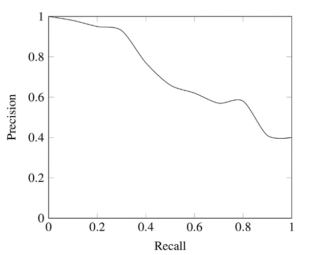
F1-Score

F1-Score comes into play when balancing precision and recall. F1-Score is the harmonic mean of precision and recall.

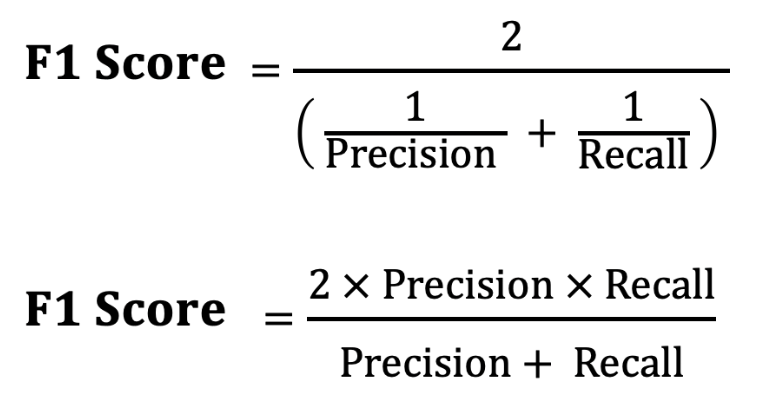
The reason for not taking the normal average here is that in a situation where recall is 1 and precision is 0 (or vice versa), the average would be 0.5, which does not give us good insight; we would end up back where we started. Instead, in the harmonic mean, if recall is 0.001 and precision is 0.999, the F1-score would be 0.001 (if it were 0, it would directly be 0). If we are looking for a balance between precision and recall, we look at the situations where the F1-Score is maximized. If we consider the doctor example I just gave, we maximize recall and minimize precision. In summary, deciding which metric to maximize is very important.

Accuracy: As everyone can guess, accuracy is the ratio of correct predictions to the total number of predictions. The opposite of accuracy is the misclassification rate, which can be expressed as (false positive + false negative) / total number of predictions, giving the error rate.

True Positive Rate: How many of the predictions we made as positive were actually positive? (True Positive / Actual Positive Cases)

False Positive Rate: How many of the cases where our actual output was negative did we predict as positive? (Too Much Positive / Actually negative situations)

True Negative Rate: How many of the cases where our actual output was negative did we predict as negative? (True Negative / Actually negative situations)

Receive Operating Characteristics (ROC) Curve & Area Under Curve

ROC and AUC are two of the most commonly used performance metrics in classification problems. It would be better to explain what ROC means through ROC.

ROC explains how well the model can distinguish between true positive rate and false positive rate. AUC gives the area under the ROC curve, which is between 0 and 1, and 0 means all predictions are incorrect. True positive rate briefly shows how many of the actual positive cases we predicted as positive, while false positive rate shows how many of the actual negative cases we predicted as positive (also known as a false alarm). So actually, we predicted positively in both cases, but the outcomes were different.

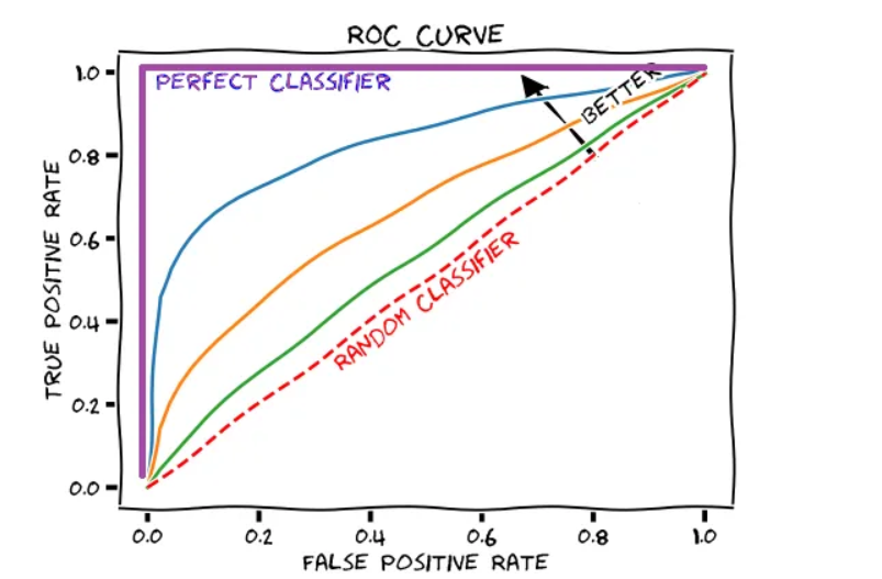
In the ROC graph, at the point (0.5, 0.5), which is the diagonal labeled "random classifier," there are models that have no classification ability. Think of the coin toss example: your null hypothesis is that heads (i.e., your positive case) will come up with a 50% probability and will not come up with a 50% probability; it doesn't make any difference. As we move up to the top left, the number of correct predictions increases. If your dataset is imbalanced, it is a more useful metric than accuracy. If negative examples suppress positive examples, AUROC can be overly optimistic; with a very simple logic, the false positive rate will be low and the true positive rate will be high because the number of true negatives in the denominator of the false positive rate will be high. That's why it's important to first look at the confusion matrix; if the situation is different, precision and recall are much more useful metrics.

Regression Metrics

R-Squared (R-Squared)

R² shows us the total variation of the regression line we have drawn compared to the actual table, which in statistics is called goodness of fit. We fit the data to a line, yes, but it answers the question of how well it performs.

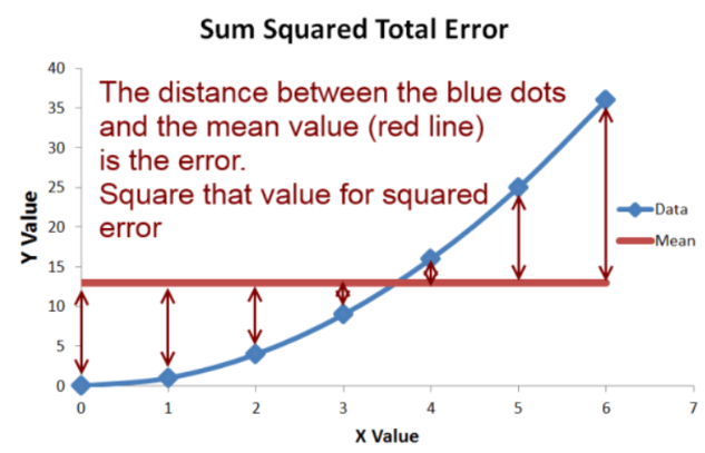
R2 measures how much better we can predict compared to the mean (average of the dataset) line above. You have a dataset and if you don't have a computer, your first guess would be to take the average and predict with the average. At this point, we find the error by taking the difference between the mean line and our data. The best R2 value is 1, and R2 values below 0.12 indicate that your model is not good. (Cohen, 1988). Normally, we assume that R2 values are between 0 and 1, but they can be negative. The negative R2 indicates that your model is obtaining a much worse fit than when you normally use the mean, meaning it is underfitting. Besides this, in a regression where we account for multiple variables (multivariate regression), we look at the adjusted-R2 value instead of R2, because R2 is often misleading.

Mean Squared Error

Mean square error simply takes the square of the distance between your regression line and the data points and divides it by the number of points. It measures the average of the squared differences between the predicted values and the actual values. In simpler terms, MSE tells you how far off your predictions are from the true values, with larger values indicating worse predictions.

Formula:

Why Make Use of MSE?

Penalizing greater Errors: MSE penalizes greater errors disproportionately by squaring the differences. Because of this, the model is strongly punished for making significant errors, which motivates it to concentrate on reducing significant deviations.
Common Metric: Because it gives a precise numerical number for a regression model's performance, MSE is often employed in statistics and machine learning. A model that fits the data better is shown by lower MSE values.

Mean Absolute Percentage Error

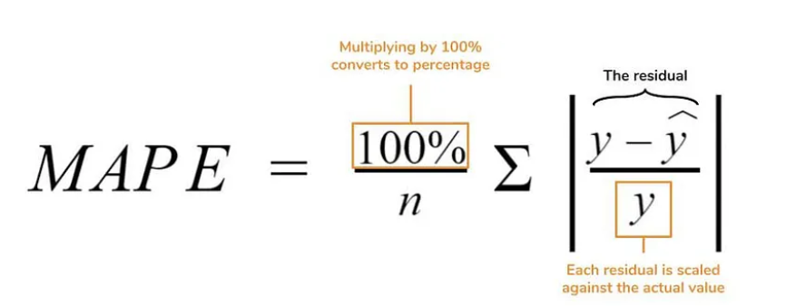
In MAPE, we subtract our predictions from the actual data, divide by the actual data, then sum their absolute values, multiply by 100, and divide by the number of data points. Although MAPE performs well against outlier data points, if your data contains 0, it will cause issues since it will also appear in the denominator. In cases where the true value is very small, the error will also be significant. Besides this, if the predicted values are lower than the actual values, the MAPE is much less than the value in the opposite situation, meaning there is a bias.

Mean Percentage Error (MPE)

The only difference between MPE and MAPE is the absence of the absolute value operation in MPE. The downside of this is that positive and negative percentage errors cancel each other out, and it does not give an idea of how much error there is in the model. The upside is that it can provide insight into whether the model is underestimating (the prediction is less than the actual value, negative error) or overestimating (the prediction is greater than the actual value, exaggeration, positive error).

Where:

• y = actual value (true value)

• y^​ = predicted value (by the model)

• n = number of data points

Thank you for taking the time to read my blog! I hope you now have a better understanding of the various error metrics used in both regression and classification problems, such as Precision, Recall, Mean Squared Error (MSE), Mean Absolute Percentage Error (MAPE), Mean Percentage Error (MPE), and more.

Feel free to leave any comments or questions below. I'd love to hear your thoughts