ML Chapter 6: Reinforcement Learning
 Fatima Jannet
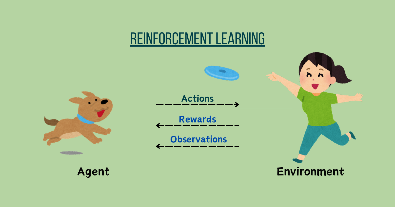
Welcome to Part 6 - Reinforcement Learning!
Reinforcement Learning is a powerful branch of Machine Learning used to solve problems by deciding actions based on past data. It's also used in AI to train machines for tasks like walking, using rewards and punishments. Machines learn through trial and error.
In this part, you will learn to implement these Reinforcement Learning models:
Upper Confidence Bound (UCB)
Thompson Sampling
Before we continue, I want to mention that the multi-armed bandit problem is not the only issue that can be solved with reinforcement learning. Reinforcement learning is actually very cool.
Reinforcement learning, for example, is used to train robot dogs to walk. Once you've created a robot dog, you can implement an algorithm inside it to teach it how to walk. You can instruct it to move its front right foot, then its back left foot, followed by the front left foot, and then the back right foot. This sequence of actions helps it learn to walk.
Alternatively, you can use a reinforcement learning algorithm to train the dog to walk in a very interesting way. Essentially, the algorithm will tell the dog, "Here are all the actions you can take: you can move your legs like this or like that, and your goal is to take a step forward." Each time it takes a step forward, it receives a reward. If it falls over, it gets a punishment.
You don't actually have to give it a carrot. A reward is represented as a '1' in the algorithm, and a punishment is a '0'. So, every time it takes a step forward, it knows it has earned a reward.
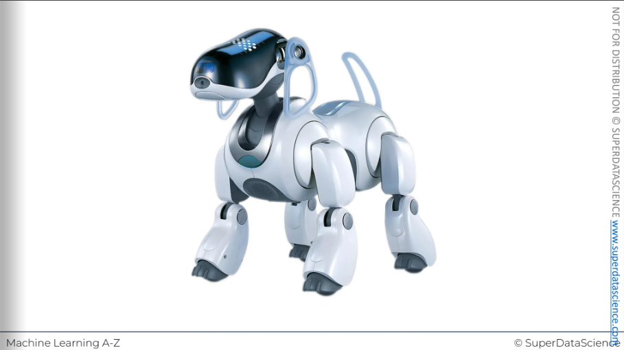
And dogs like that can actually learn to walk on their own. You don't need to program a specific walking algorithm into them; they'll figure out the steps they need to take by themselves. Isn’t it cool?
but that's more related to Ai than just ml. We won't cover training robot dogs to walk here. Instead, we'll discuss the multi-armed bandit problem, a different application of reinforcement learning.
The Multi-Armed Bandit Problem
A one-armed bandit is a slot machine. But why is it called a bandit? Well, because these machines were known as one of the quickest ways to lose your money in a casino. They had about a 50% chance of tking your money. So, you would often earn less than you actually won, with a roughly 50-50 chance of either winning or losing money.
However, there was a time when a bug was introduced, causing players to lose even more frequently than 50%. That's why they're called bandits, making it one of the fastest ways to lose money. Hence, the name "one-armed bandit."
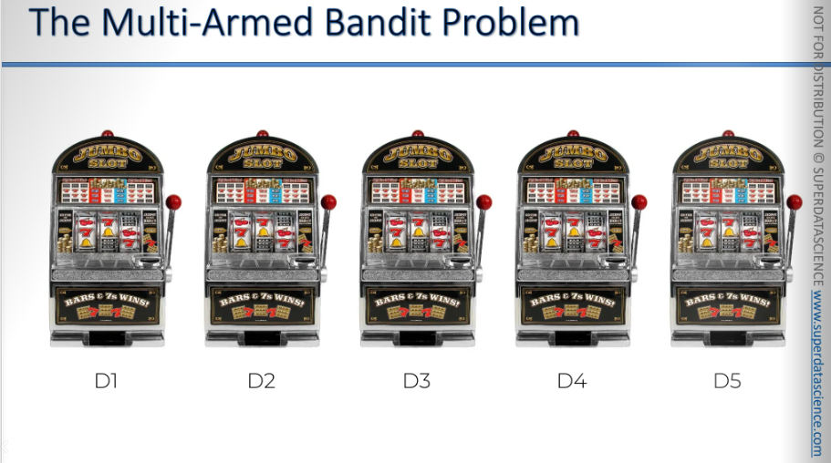
Now, what is the multi-armed bandit? The multi-armed bandit problem is the challenge faced when a person encounters a whole set of these machines, not just one, but maybe five or ten. [Programming examples often use ten machines, but we won't focus specifically on these machines. This is the historic problem]
You'll soon see that there are many other applications for the multi-armed bandit problem. Although it's called the multi-armed bandit problem, it's actually used to solve many other issues as well. So, basically, you're faced with a challenge: you have five of these machines. How do you play them to maximize your return from the number of games you can play?
Let's say you've decided to play a hundred or a thousand times, and you want to get the most out of it. How do you figure out which machines to play to maximize your returns?
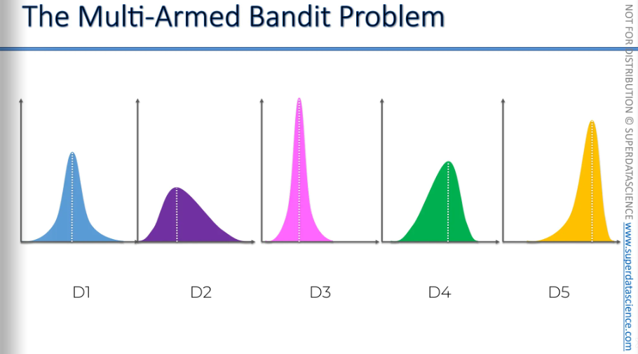
To explain the problem further, we need to mention that each machine has a distribution behind it. This means there's a range of outcomes from which the machine picks results. Each machine has its own distribution, and when you pull the lever, it randomly selects a result from its distribution. This determines whether you win or lose, and how much you win or lose. Basically, you lose the same amount you put in the coin, but the machine tells you if you win or lose based on its built-in distribution.
The problem is that you don't know these distributions, right? And they are assumed to be different for each machine. Sometimes they might be similar or the same for some machines, but by default, they are different. Your goal is to figure out which of these distributions is the best for you.
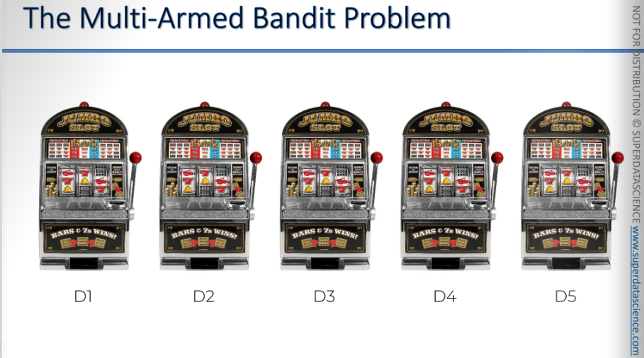
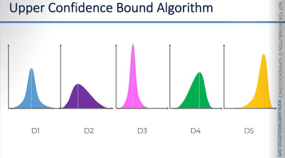
Let's take a look. We have these distributions, right? For example, we have five machines with five different distributions. Just by looking at them, you can see which is the best machine. Obviously, the one on the right, the yellow one, is the best because it's the most left-skewed, meaning it tails on the left. It has the most favorable outcomes with the highest mean, median, and mode. If you knew these distributions in advance, you would obviously choose the fifth machine and bet on it every time because it has the best distribution. On average, you would get the best results.
But you don't know that in advance, and your goal is to figure it out. It's like a mind game. You can't waste your time thinking because the more time you lose, the higher the chance of spending money on the wrong one becomes. There are only two factors:
exploration
exploitation
So you need to explore the machines to find out which one is the best. At the same time, you should start exploiting your findings to maximize returns.
There's another mathematical concept behind all of this called regret. Regret occurs when you use a method that isn't optimal. The machine on the right is the optimal one. Whenever you use a non-optimal machine, you experience regret. This can be measured as the difference between the best outcome and the non-best outcome, including the opportunity cost of exploring other machines. The longer you explore non-optimal machines, the higher the regret. However, if you don't explore long enough, a suboptimal machine might seem like the optimal one.
For example, if we don’t explore enough we might take the green one as the optimal machine (it got a quite good return) whereas the yellow one is the best one. The goal is to find the best one, exploit the best one using the least amount of money.
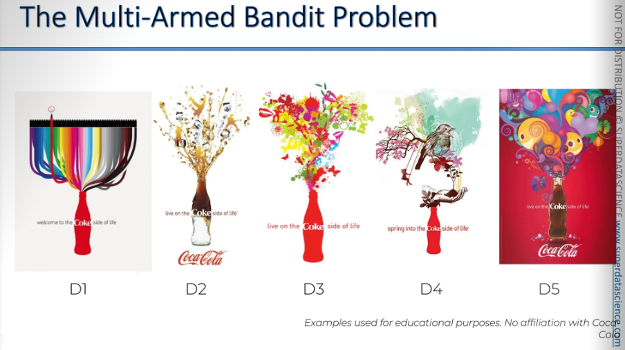
Let's take a look at some ads. This is going to be fun.
Disclaimer: there is no affiliation with Coca-Cola. These examples are used purely for educational purposes.
Let's say Coca-Cola wants to run a campaign called "Welcome to the Coke Side of Life." If you search for this campaign online, you'll find they created hundreds of different ads. Here's an example: these are some images I found on Google. They might even be drawn by people, but let's assume they are legitimate ads intended for the campaign.
Our goal is to find out which ad works best. We have options: number one, number two, number three, number four, and number five. We want to determine which ad performs the best to maximize our returns. Right now, we don't know which ads are the most effective. There is a distribution behind it, but we'll only understand it after thousands of people view these ads and either click on them or not.
This is quite similar to the example we're going to explore.
Upper Confidence Bound (UCB)
Basically, our task was to find out the best algorithm behind the bandits through exploration and exploitation making sure to invest least amount of money. Now the modern application of this process is advertising. So, if you have 5, 10, 50, or even 500 different ads, how do you figure out which one is the best? You could run an AB test and use those results, but that means you're exploring and exploiting separately. This approach can be costly and time-consuming. Instead, we want to combine exploration and exploitation to quickly reach the best result and maximize our efforts.
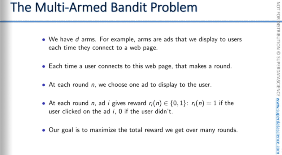
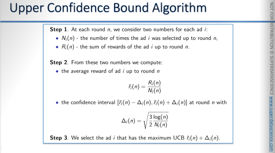
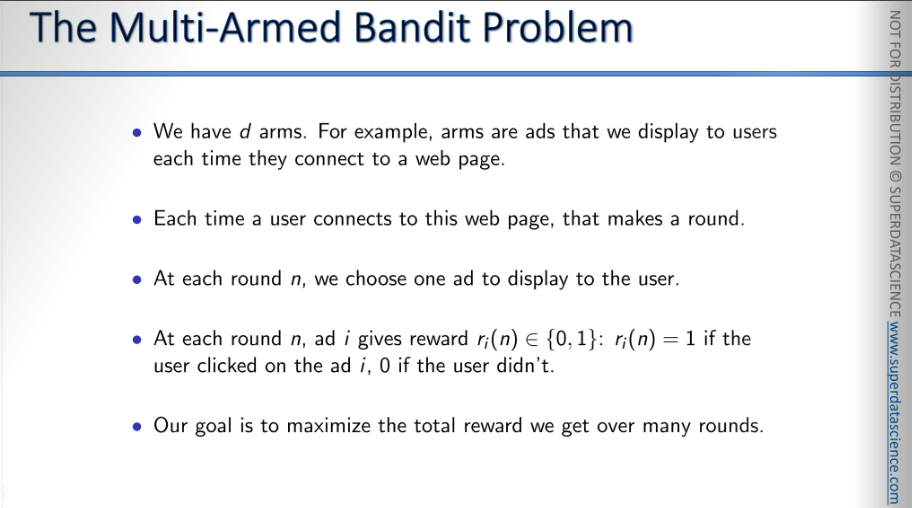
Go through this quickly. We have D arms, which are ads shown each time a user visits a webpage. Each display is a round. For each round "n" we choose which ad to show. Usually, only one ad is displayed, like pulling one arm on a one-arm bandit. Ad "ri" gives a reward of one if clicked, or zero if not. Our goal is to maximize the total reward over many rounds. That's it.
And this is how the upper confidence bound algorithm works. I’m not going into details here cause we are going to code on this formulas. Let’s get into the intuition part on how does it work? When the algorithm runs, what’s happening in the background?
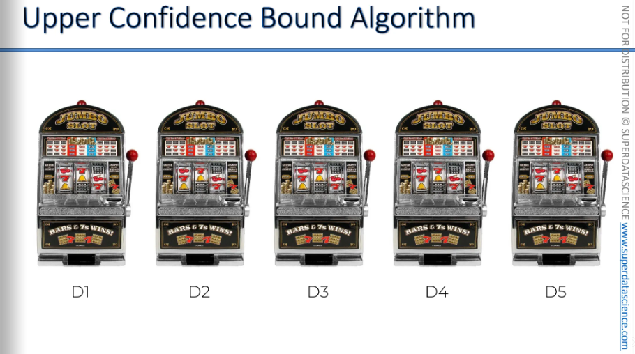
These are our slot machines, or one-arm bandits, and each one has a distribution behind it. By looking at them, we can't tell which one is the best. But let's say, for the sake of argument, we know the end result.
Let’s say these are the distributions behind it. seeing them, you know that the yellow one has the best return and you would constantly bet your money on it. But we don’t know that. And we want to find that out by playing these machines or using the ads we're running to see which one gets the most clicks. We don't have the time or money to explore this before the actual campaign starts. We want to do it during the process. So, how do we do that?
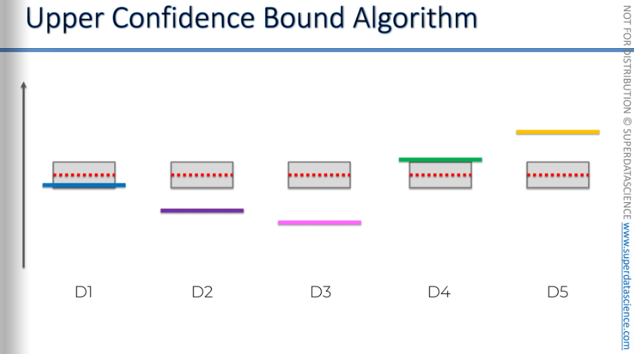
We’ll we will transfer these values into x and y axis.
So here it is. These blue, purple, pink, green, yellow lines are the distributions (not the heights). But as we don’t know what will they return, let’s put a same distribution for all of them, which as you can see, the red dotted line over here. The algorithm now will use formulas to create a confidence band. This band is designed in such a way that, it includes the actual or expected return with high certainty. Again, we don't know the distribution; everything is unknown. It's time to pick an ad.
Let's say we pick the pink one. The we pull the level, or or we place that ad. So we display the ad and check if the person clicked on it or not.
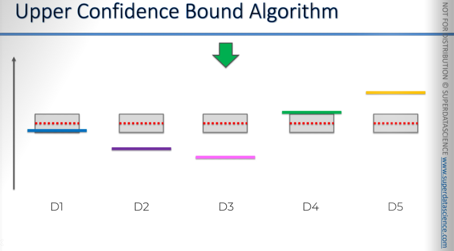
In this case, the person didn't click on it, so the red value goes down. The red value represents the observed average. As the mark drops down, the confidence boundary shrinks too. Although it's not visible here, the return rate decreases.
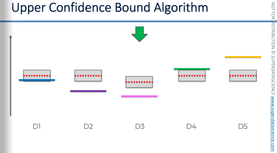
Well, now we have 4 other options left. We've picked the green one here and did the same procedure. So, the ad is shown, and a person either clicks or doesn't. This impacts the average we've measured so far. The empirical average or you've pulled the lever, shown by the red line, changes based on whether you win or lose.
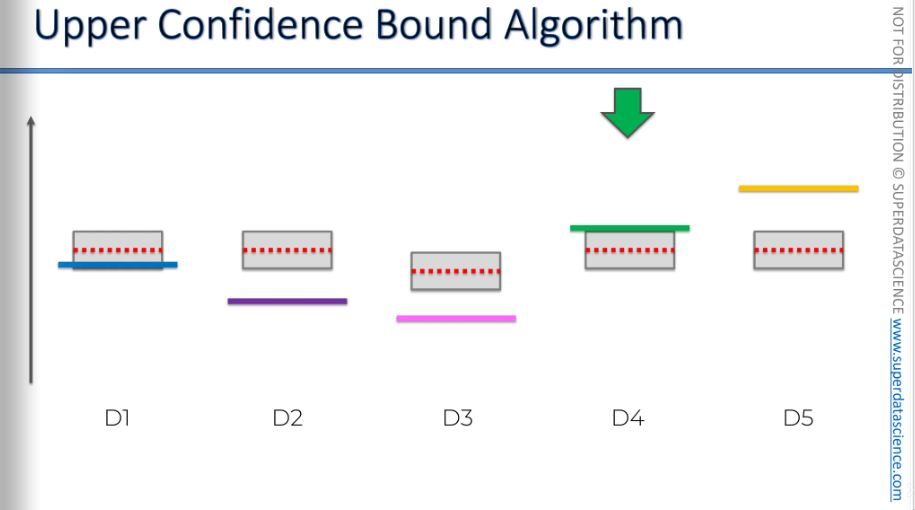
As you can see now, this machine is suddenly above all the other machines, right? So, if this were the end of the iteration, that would be it. We would assume from here that this is the best machine and start using it, making this algorithm completely useless.
But we shouldn't forget about the second thing that happens. When we get an additional observation in our sample, we become more confident in this interval and these confidence bounds. Their only purpose is to include the actual expected value, wherever it is. We don't know exactly where it is, but they indicate that this green value is somewhere inside this box. With the new observation, our sample size is larger, making us more confident in the overall picture for this machine. As a result, the confidence bounds decreased. Now, as you can see, it's no longer the top machine because, even though it went up(red mark), the confidence bounds went down(not visible here). Now, we will look for the next highest confidence bound.
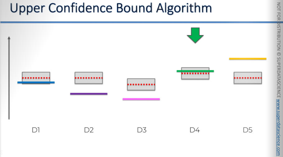
And just look at any one randomly for now, this blue one.Here, even though the red line is above the blue line, according to the law of large numbers, you'd expect them to eventually converge. But sometimes, it can randomly happen that it goes the other way, right? Things like this can occur. It's all about probability. So, basically, it might even go up. There we go, it went up, even though the blue line was below the red line. It can happen just by chance, right? In the long run, it will converge, but on a random occasion, it can go up or in any direction. And again, we got another element in the sample, so the confidence bands converge. Okay, so we kind of get the picture of what's going on here.
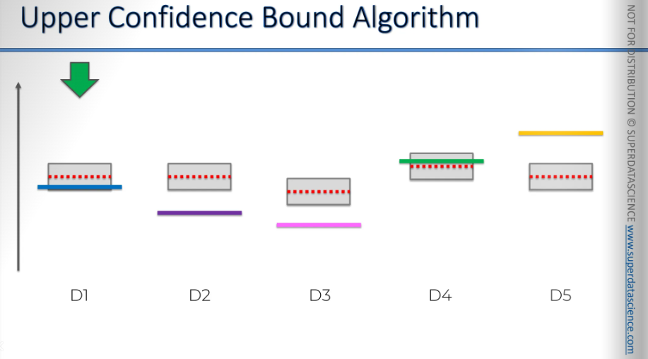
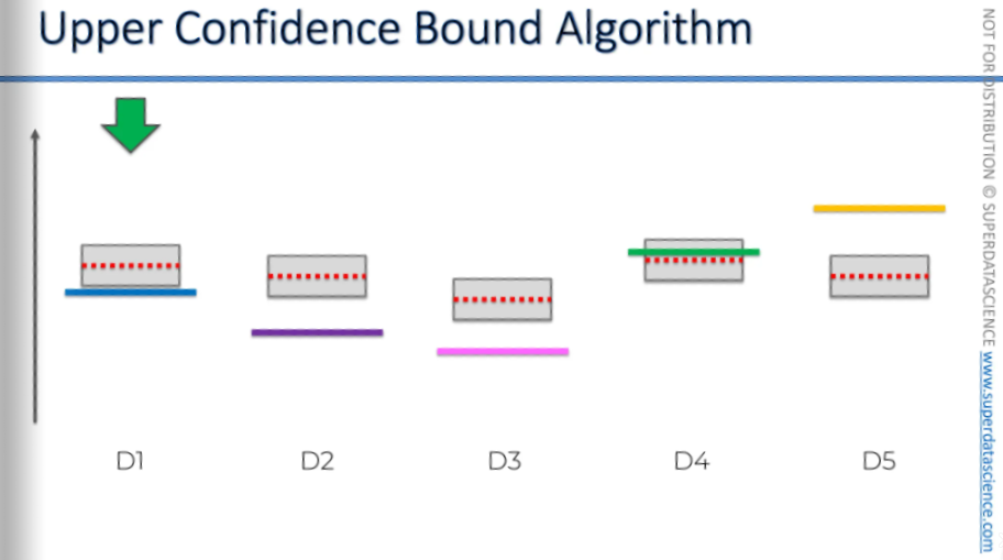
So, now we're going to pick the next one. Then we conduct the trial and complete the round. What happens when the person clicks on the ad? Do we win money from the slot machine, and does it go down?
Probably not.
We didn't click on the ad and didn't win money from the slot machine. So, the average of our observations goes down, moving closer to the expected value, and the confidence bounds also decrease.
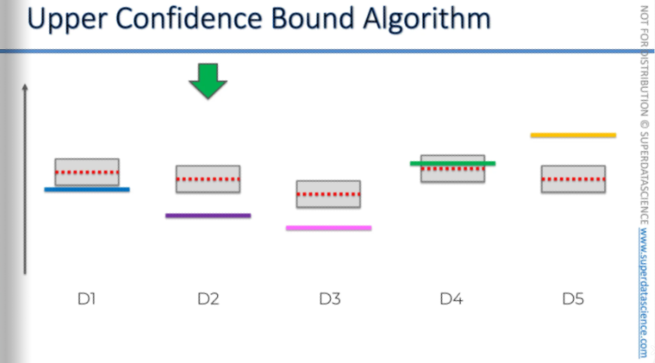
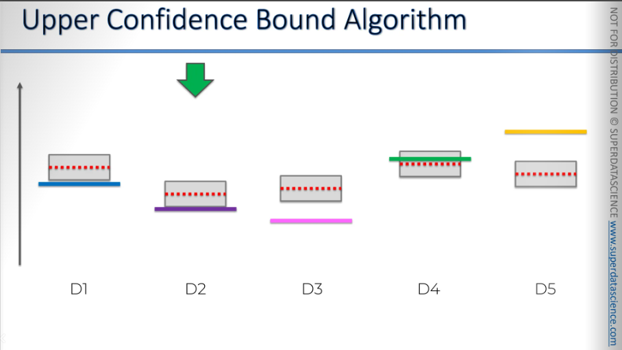
The next one is the yellow one. Now, since we know the final outcome, we understand that this is the best choice, right? We know this is the best ad or the best slot machine to use. However, this insight was given to us just for the sake of this exercise. The person using this algorithm, or the algorithm itself, doesn't know this. So, unknowingly, it's starting to exploit the best option right now. Once again, it goes up, which is good, and the confidence band goes down. As you can see, it's still the best choice.
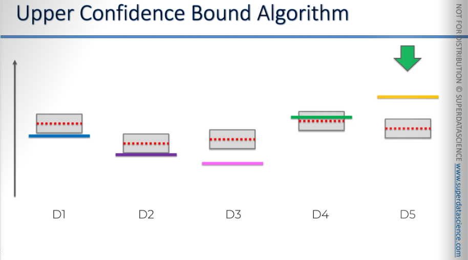
All right, we'll use this one again, and it gets closer, but the confidence bound decreases. Remember, this is just for illustration.
Of course, it won't decrease that much from just one observation, but we don't want to sit through a thousand iterations. This is just to show the overall picture.
So, even though we're using the best option, by doing so, we're reducing the confidence bound, which allows other options to have a chance.
As we increase the sample size, it gives other options, machines, or ads a chance, so we're not biased towards what we think is the best or optimal choice.
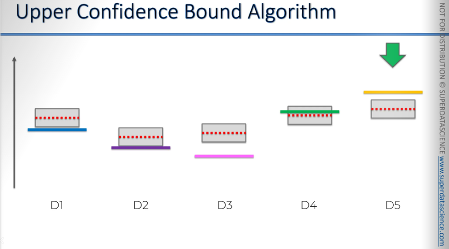
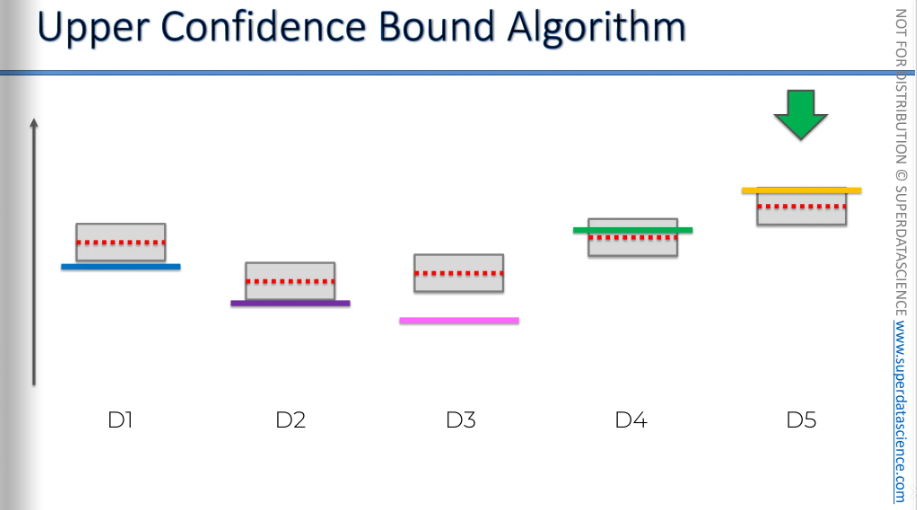
Now, as we move on to this one, the same thing happens: it gets closer, and the bounds decrease.
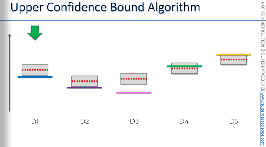
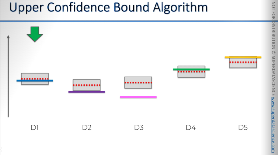
We move on to the next one, and the bounds decrease.
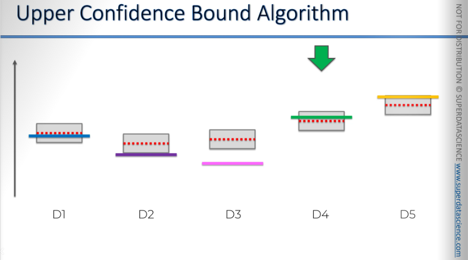
Then we move on to this one, and the bounds decrease again.
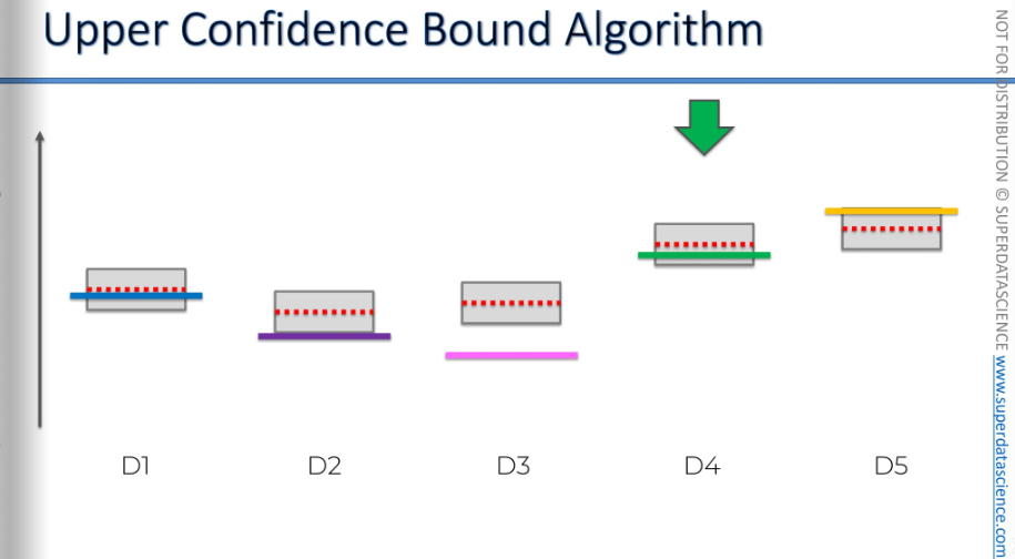
And again, this one might get closer, and the bounds decrease.
Even though we were very close to finding the solution, the bounds decrease significantly.
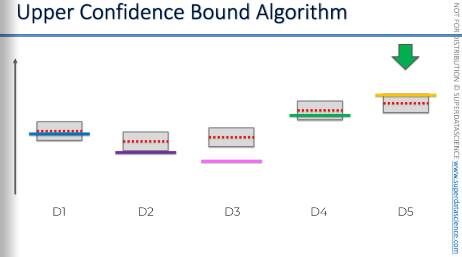
You'll see this in practical applications and tutorials that follow. Sometimes, after using the best option for a while, the algorithm will switch to a less optimal option because the bounds keep decreasing.
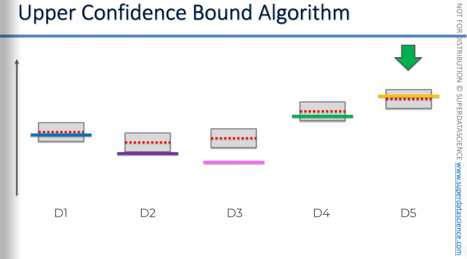
Then we'll use this one, the bounds will decrease, and now we're back to the best one, and the bounds decrease again.
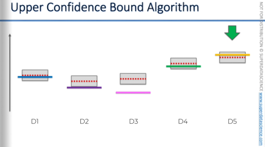
We'll keep using this one because we've found it's the best.
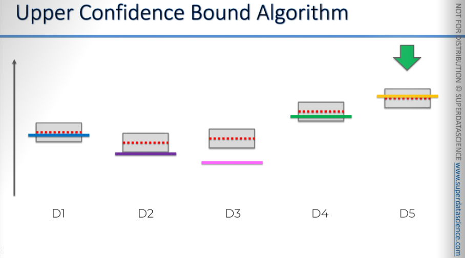
This is the core idea behind the upper confidence bound algorithm. It solves the multi-arm bandit problem in a way that's more advanced than just picking randomly or running an A/B test and then choosing the winning option.
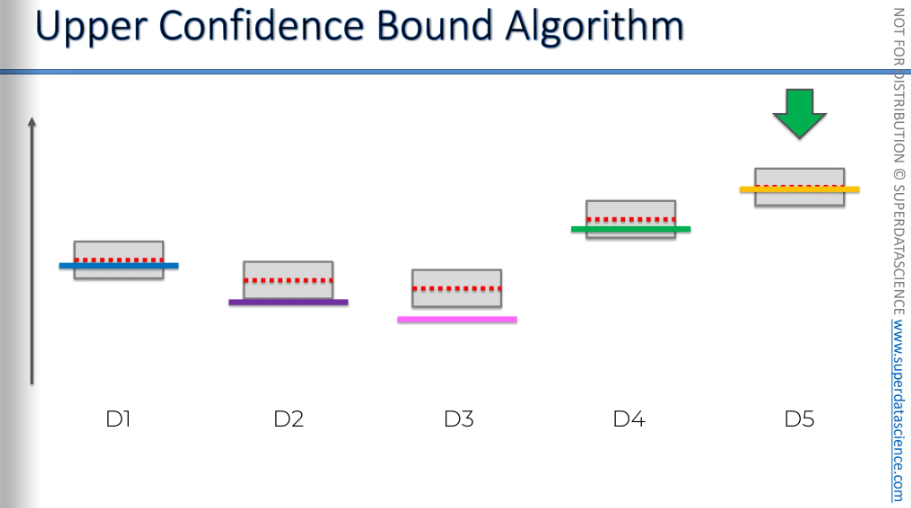
So, if you're in advertising, running campaigns, or facing similar problems, remember the upper confidence bound algorithm. You can apply it in your work too. It's a very powerful algorithm.
UCB in Python steps
Get your code and datasheet here
Upper Confidence Bound, It's one of the most exciting areas of machine learning because it's closely related to artificial intelligence. Here we will be making some programs that takes action just like a robot.
You remember that SUV? The brand new luxury SUV that the car company was trying to target better using classification. This time, we're going to optimize online advertising, which means we'll find the best ad.
About the dataset:As I mentioned, we're continuing the story of the car dealership selling the new SUV. We've optimized targeting with classification, and now we'll optimize the click-through rate for the ads. The advertising team created 10 different ads, each with unique designs, like the SUV in a mountain, a futuristic city, a charming city, on the moon, or in a countryside cornfield. The team wants to know which ad will convert best.
We have 10 different ads to show to users online. When users visit a website or search engine, an ad appears at the top of the page. Each time a user connects, we show one ad and record if they click "yes" or "no." UCB selects which ad to show. If a user clicks, we record a "1"; if not, a "0." Then, when a new user connects to the webpage, the algorithm will select an ad for this new user. We repeat this for 10,000 users, and that's what the dataset is about.
[Please note: In reality, what happens is that users connect to the webpage one by one, and we show each of them an ad. Everything occurs in real-time, making it a dynamic process. It's not a static process with a dataset recorded over a specific period. It's happening in real-time.
To simulate this, I would need to create 10 real ads, open a Google AdWords account, and show them to real users. But this is costly and could mislead users, as I'd need to sell a car, which isn't feasible. So, I rely on a simulation, which is what the dataset provides. We can't know this in reality, which is why this dataset is a simulation. It's the only way to run the UCB or Thompson sampling algorithm without a real advertising campaign.]
Importing
The first steps are to import the libraries and the dataset. For reinforcement learning, we don't need to create a matrix of features or a dependent variable.

Implementing UCB
Time for implementation. We will follow these three steps:

Make sure to understand the indexes and variables here.
#step1
The total number of users is stored in the variable N.
The number of ads is stored in the variable d, which is 10.
Create a variable to keep track of the selected ads over the rounds. It starts as an empty list and will grow to 10,000 items, representing the ads chosen for 10,000 users.
Initialize another variable as a list of 10 elements, all set to zero.
The last variable is the total reward, which is the sum of all rewards received in each round. In the dataset, zeros and ones represent these rewards. If a user clicks the ad, we get a reward of one; if not, we get zero.
#step2
Start a for loop to go through all 10,000 rounds.
Begin by picking an ad. We'll start with the first ad, which is ad number one. Since we're using indexes, this ad's index is zero. So, we'll set the variable
adto zero.Add a second for loop to check each ad one by one.
To find the highest upper confidence bound, we need to compare the upper confidence bound of each ad.
The second for loop will run from 1 to 10.
Implement the steps mentioned in step 2.
If the ad hasn't been picked yet, we need to choose it. This ensures the denominator Ni(N), which counts how many times ad I was picked, isn't zero. This is important so we can calculate the average reward and the upper confidence bounds.
To make sure this ad gets picked, we set its upper bound to a very high value in the second for loop. This way, it will be the highest upper bound and will be chosen. At the end, we always pick the ad with the highest upper confidence bound.
The trick is to set this variable to a very high number if the ad hasn't been picked yet. If we're not in this situation, we want the variable to be a very high number, like infinity. But since we can't use infinity directly, we use a very large number, like 1 times 10 to the power of 400. This is a common trick in Python to mimic infinity.
import math

# Step 1: Initialize variables
N = 10000  # Total number of rounds (number of users/observations)
d = 10  # Number of ads/options to select from
ads_selected = []  # List to store selected ads in each round
number_of_selections = [0] * d  # List to store the number of times each ad has been selected
sums_of_rewards = [0] * d  # List to store the cumulative rewards for each ad
total_reward = 0  # Initialize the total reward to 0 as no rewards are collected in the first round

# Step 2: Implement UCB algorithm
for n in range(0, N):  # Iterate through each round
    ad = 0  # Initialize the ad to be selected in the current round
    max_upper_bound = 0  # Initialize the maximum upper bound

    # Iterate through each ad to calculate the upper confidence bound (UCB)
    for i in range(0, d):
        if number_of_selections[i] > 0:  # If the ad has been selected at least once
            # Calculate the average reward for ad i
            average_reward = sums_of_rewards[i] / number_of_selections[i]

            # Calculate the confidence interval (Δi(n)) for ad i
            delta_i = math.sqrt(3/2 * math.log(n + 1) / number_of_selections[i])

            # Calculate the upper bound for ad i
            upper_bound = average_reward + delta_i
        else:
            # If the ad hasn't been selected, set its upper bound to infinity (ensures selection)
            upper_bound = 1e400

        # Update the ad selection if the current ad's UCB is greater than the max
        if upper_bound > max_upper_bound:
            max_upper_bound = upper_bound
            ad = i  # Update the ad index to the current ad

    # Record the selected ad for this round
    ads_selected.append(ad)

    # Update the number of selections for the selected ad
    number_of_selections[ad] = number_of_selections[ad] + 1

    # Get the reward for the selected ad in the current round (assuming rewards are from a dataset)
    reward = dataset.values[n, ad]  # Replace `dataset.values` with your actual data source

    # Update the cumulative rewards for the selected ad
    sums_of_rewards[ad] = sums_of_rewards[ad] + reward

    # Update the total reward collected so far
    total_reward = total_reward + reward
Visualizing the results
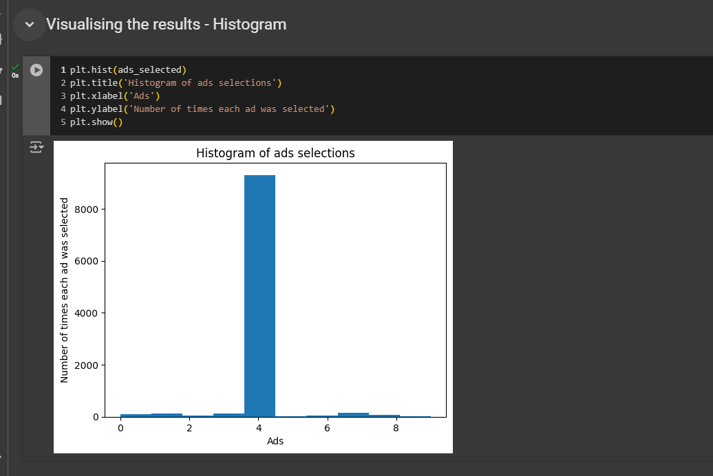
This histogram will show how many times each ad was selected.
On the X-axis, we will have the different ads, ranging from zero to nine, since we use indexes that start at zero.
On the Y-axis, we'll display the number of times each ad was selected.
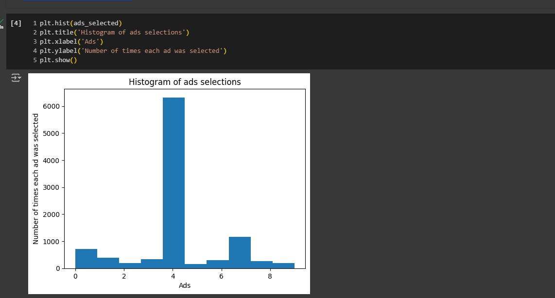
Indeed, the ad with index four, which is ad number five, was clearly selected the most. This means it had the highest click-through rate. In our business case study, this corresponds to the most attractive ad, featuring the most appealing image of the car that will likely sell the most to future customers.
It's not quite over.We should experiment to see how many rounds the UCB algorithm actually needs to identify the ad with the highest CTR.
To check this, we can change the value of N from 10k. Let's try running it with 5k and rerun everything to see if UCB still picks the correct one. And yes, it does! No we are going to replace N with 500.
You will notice that you get two identical bars in your histogram. That's what I'm referring to. You see, 500 rounds are not enough for the UCB algorithm to identify the best ad.
We are diving into the exact same data set with Thompson sampling! Get ready to compare and see the magic unfold. Let's jump into this in the next section!
Thompson Sampling
Recap: we're using this algorithm to solve the multi-armed bandit problem with several slot machines, each with an unknown distribution (D1 to D5). We need to play these machines to find the best distribution and exploit it. Our goal is to maximize returns while balancing exploration and exploitation.

A quick summary of the multi-armed bandit problem is as follows:
You want to find out which of these ads performs the best, but you don't have the time, funds, or resources to conduct an A/B test. You want to determine this quickly. That's when you would use one of the algorithms we're discussing in this part of the course.
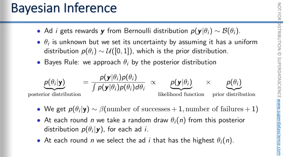
Here we have some complex mathematics, Bayesian inference, distributions, posterior probability, and beta distributions. We're not going to dive deep into this now.
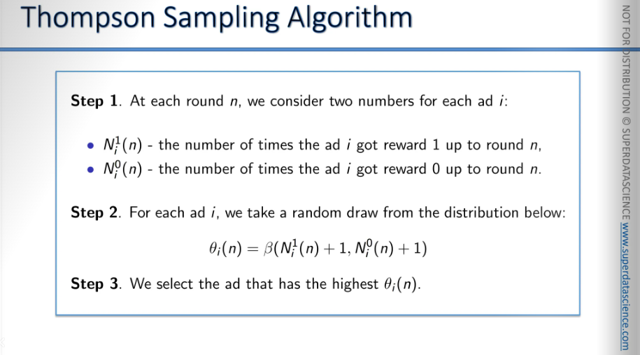
These are the actual steps that you are gonna be using.
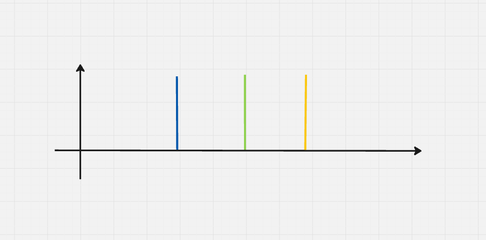
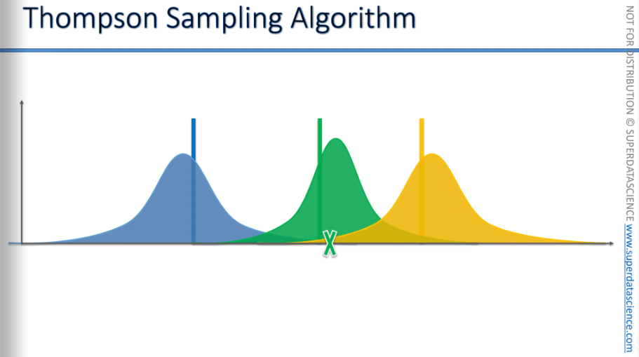
Here, y axis is the return which we expect from the bandits. Also, instead of 10 bandits, we will look at 3 here cause 10 will clutter the chart a lot, i don’t wanna do this.
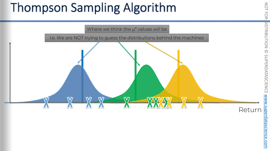
The vertical lines (blue, green, yellow) represent the expected return for each of the machines. Each of the representation has a distribution behind it, the amount of money. Even the algorithm itself doesn't know this information, right?
Now we need some trial runs. Can you see the cross marks? that are the trials we have run. And based on the trials, the Thompson algorithm will generate a distribution. Now we have some sort of perception of the current state of things. Therefore, we have created a distribution showing where we believe the actual expected value might be. We are creating an auxiliary mechanism for us to solve the mission. The values could be anywhere inside the distribution (though it's very likely to be at the top)
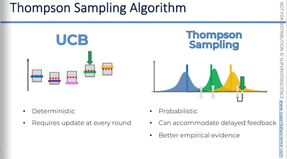
The Upper Confidence Bound (UCB) was a strict, deterministic algorithm. We chose whichever had the highest upper bound confidence. But the Thompson algorithm is a probabilistic perception. It creates a distribution that shows the value could be anywhere within it.
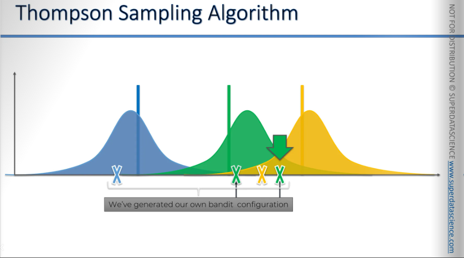
So these bars (vertical colored lines) represent the actual expected returns for each machine, but the algorithm doesn't know them. The algorithm has created a distribution which allows to kind of have a guess where the value could be. So, now the algorithm will call the distributions and pull a value from it.
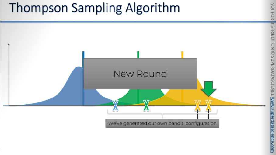
Guess what we have done? We have constructed our own bandit configuration. We have created a hypothetical machine in our own virtual world. Now we will solve the problem.
We will pick the green machine cause it has the highest expected return out of the three. We have selected the green machine in our virtual world, now we will pull the lever of the green bandit in our real world. And it will give us a value. The value could be somewhere near or far from the actual value. Let’s say the value is the green cross (without the arrow on top of it). This is a new information to the algo.
Now the algorithm will adjust it’s perception of the world.
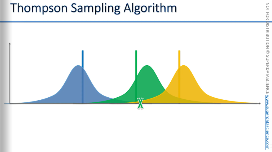
Look carefully, the algorithm has slightly shifted the green distribution to the left due to it’s new perception. Also it has became narrower because now it has more information. Each time we get new information, our distribution will get more and more refined.
Now we'll do the same thing again for another distribution. We generate or select some values. We've created our own bandit configuration in our virtual or hypothetical world. Out of these three, we need to choose the best bandit, which is the yellow bandit.
Now, we will pull the lever of the yellow bandit in the real world, or the algorithm will do it. This action will trigger the distribution behind the yellow bandit and give us a value. The new cross (without the arrow on top) represents the actual value we received in the real world.
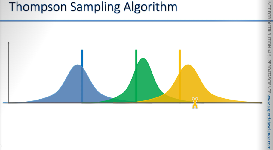
Now we're going to incorporate that value into our understanding of the world, and our perception will change and adjust accordingly.
There we go.
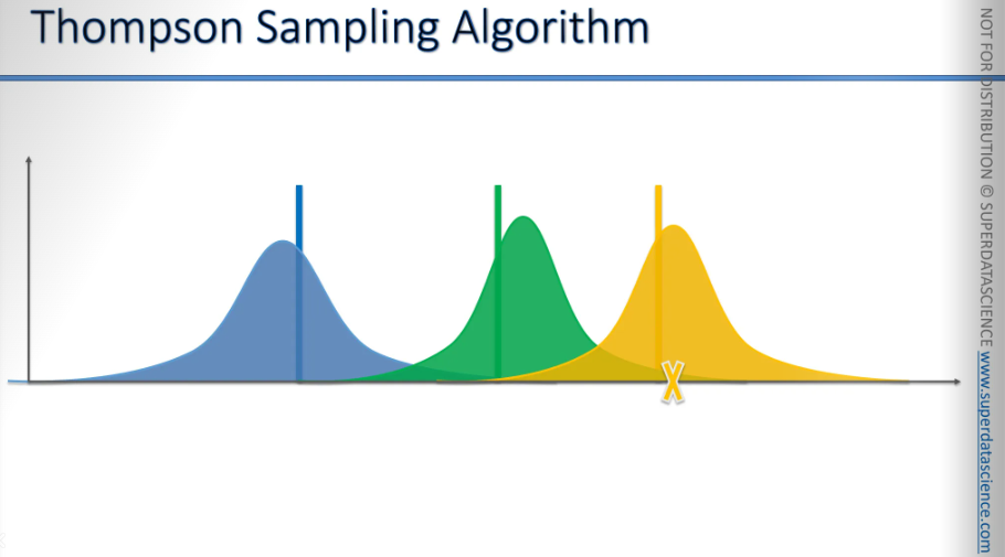
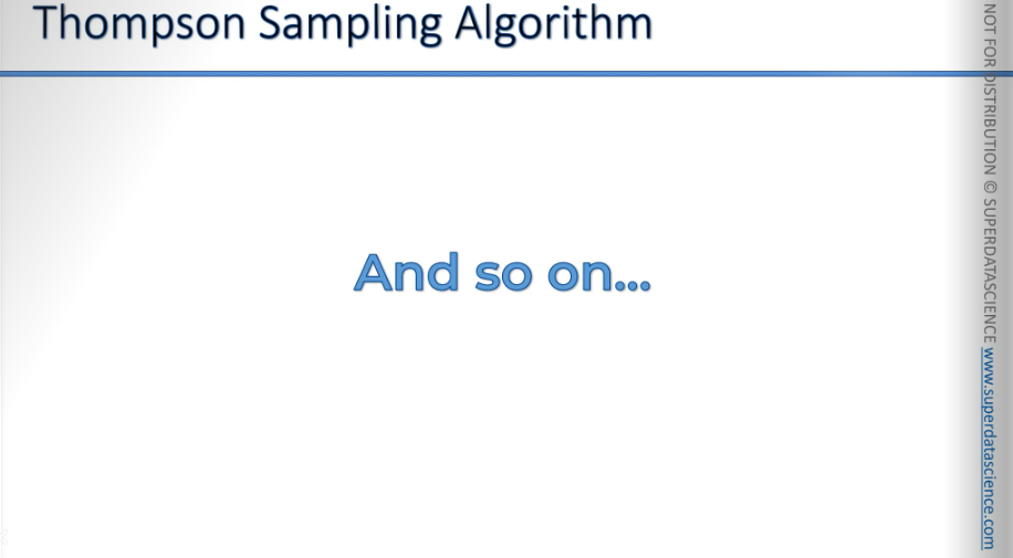
And so, we will continue this process until we reach a point where we've significantly refined the distributions, and the picture looks like this. They may become even more refined over time.
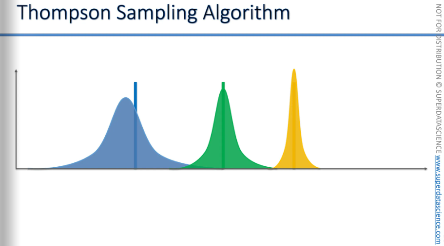
Now we have completed our exploration and it’s time to exploit
Algo comparison: UCB vs Thompson Sampling
I will just highlight the main pros and cons here.
UCB
Very straightforward, very deterministic, only one round. You choose the one with higher UCB.
The UCB needs updating every round. After pulling the lever and getting a value, you must update immediately to move to the next round. Without this adjustment, nothing changes, and you'll be stuck.
Thompson Sampling
It’s probabilistic, distribute perceptions, refines through multiple rounds, always different.
It can handle delayed feedback. Even if you only get the results after 1,000 rounds, the algorithm will still work. This is because, even without updating your understanding of the world, you'll still get a new set of hypothetical bandits. You'll generate a new expected return for each bandit since they are created in a probabilistic way.
Better empirical evidence: You are gonna see it beating the UCB in the code implementation.
Thompson Sampling in Python steps
Get your code and datasheet here.
import random  # Import the random library for generating beta distributions
N = 10000  # Total number of rounds (users visiting the ads)
d = 10  # Number of ads
ads_selected = []  # List to store which ad was selected at each round

# Initialize lists to keep track of the number of rewards for each ad
numbers_of_rewards_1 = [0] * d  # Number of times reward 1 (click) was obtained for each ad
numbers_of_rewards_0 = [0] * d  # Number of times reward 0 (no click) was obtained for each ad
total_reward = 0  # Total accumulated reward

# Iterate over all rounds
for n in range(0, N):
    ad = 0  # Initialize the selected ad for the current round
    max_random = 0  # Maximum random beta value observed for this round

    # Loop through all ads to find the ad with the highest beta distribution value
    for i in range(0, d):
        # Generate a random value from a beta distribution using the rewards so far
        random_beta = random.betavariate(numbers_of_rewards_1[i] + 1, numbers_of_rewards_0[i] + 1)
        if random_beta > max_random:
            max_random = random_beta  # Update max_random with the higher beta value
            ad = i  # Select the ad corresponding to the highest beta value

    # Append the selected ad to the list of selected ads
    ads_selected.append(ad)

    # Retrieve the reward (1 or 0) for the selected ad from the dataset
    reward = dataset.values[n, ad]  # Replace `dataset` with your actual dataset variable

    # Update the reward counts for the selected ad
    if reward == 1:
        numbers_of_rewards_1[ad] += 1  # Increment the count of reward 1
    else:
        numbers_of_rewards_0[ad] += 1  # Increment the count of reward 0

    # Update the total reward
    total_reward += reward
Remember UCB worked well will 10k samples, then 1k samples. But it did’’t showed the best result when N was 500.
Well, as for the Thompson, after tryin 10k → 1k → 500 : It still showed the best result. And thus Thompson algo beats UCB
I haven't included different histograms for various values, but feel free to try it out on your own. See you in the next blog: NLP!
Subscribe to my newsletter
Read articles from Fatima Jannet directly inside your inbox. Subscribe to the newsletter, and don't miss out.
Written by
