ZeRO and PyTorch FSDP (Fully Sharded Data Parallelism) are powerful set of memory optimization techniques that enable effective training of large models with trillions of parameters. They form the foundation of large language model (LLM) training today.

In this post, we’ll focus primarily on ZeRO-DP (ZeRO Data Parallelism), drawing from the original ZeRO paper. Much of the analysis should also be applicable to PyTorch FSDP, though. While the paper provides a thorough explaination of ZeRO’s design and implementation, it assumes readers to have some familiartiy with distributed training, and glosses over certain details that I personally find essential for grasping the mechanism.

The basic idea behind ZeRO-DP is to partition the training model states and distribute them onto multiple GPUs, while introducing as little communication overhead as possible. This unlocks the possibility for training a much larger model and achieving a superlinear speedup relative to the number of GPUs.

Before diving into ZeRO-DP, we should first examine the GPU memory (vRAM) consumption in an ML model. Say we are training a model with 1.5B parameters (weights), while it might be tempting to think this takes 1.5B x 4 = 6GB memory for storage (4 byte per f32), it is far from the truth.

Today, large-scale model training neither uses f32 for its parameters, nor are parameters the only state stored on the GPU. The model states consist of three parts: the parameters (p), the gradients (g) and the optimizer states (os). For memory and computational efficiency, both parameters and gradients are stored as 16-bit floating points (normally bf16). As for the optimizer states, a commonly used optimizer is Adam, which stores an f32 copy of the parameters, as well as momentum and variance (no need to worry about their meanings here—just know that both momentum and variance have the same shape as the parameters). This is known as mixed precision training, with the optimizer states consuming the majority of the vRAM.

Back to our example, we can see that for the 1.5B model, the vRAM it actually needs is 24GB.

$$\underbrace{1.5B \times 2}_{p} + \underbrace{1.5B \times 2}_{g} + \underbrace{1.5B \times 4 \times 3}_{os} = 24GB$$

ZeRO-DP is a direct answer to these three states’ partitioning strategy. Figure 1 from the paper shows ZeRO-DP’s three optimization stages. Ψ denotes the model size (number of parameters), K denotes the memory multiplier of the optimizer states (e.g. 12 for Adam optimizer), and Nd denotes the DP degree (i.e. number of GPUs).

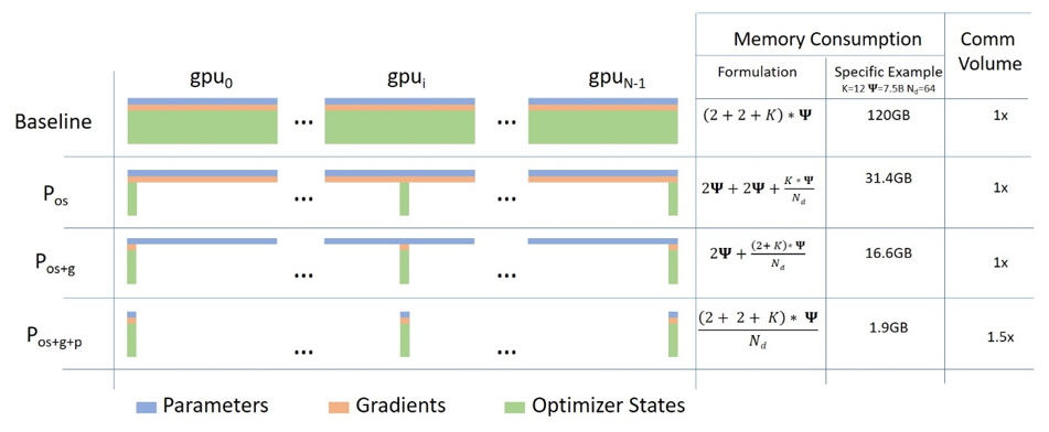
• Baseline: This is the standard data parallelism (DP). During training time, each GPU stores an identical copy of the entire model states. Compared to other parallelizing strategies (tensor or model parallelsim), this incurs the least amount of inter-GPU communication volume. However, because the model must fit into a single GPU, standard DP severely limits the model scale.

• ZeRO Stage 1 (P_os): Stage 1 groups the optimizer states equally into Nd partitions. Each GPU worker process only stores and updates 1 / Nd of the total optimizer stats, thus updates only 1 / Nd of the parameters. Still taking Adam as the optimizer (K=12), as Nd goes larger, this would eventually result in a 4x memory reduction. It has the same amount of communication volume as DP does.

• ZeRO Stage 2 (P_os+g): Stage 2 groups both the optimizer states and gradients into Nd partitions. Because each GPU worker only updates 1 / Nd of the parameters, it would only need the corresponding 1 / Nd gradients, too. Stage 2 also has the same amount of communication volume as DP does.

• ZeRO Stage 3 (P_os+g+p): All three states are partitioned, meaning the memory reduction is linear with Nd. Compared to DP, ZeRO stage 3 incurs a 50% increase in communication volume.

This leaves us with two questions:

1. Can we partition the training computation to multiple GPU devices?

2. If so, what kind of communications are neecessary among the GPU devices to ensure the integrity and consistency of the full model?

Computation Analysis

Model parameters (P) typically consists of multiple layers of tensors, where the outcome of one layer is fed into the next. The computations between these layers are independent: once a layer produces its output, the memory used by that layer can be released. This temporal independence is a key attribute to enable model partitioning, as pointed out in the paper:

ZeRO-DP … uses a dynamic communication schedule that exploits the intrinsically temporal nature of the model states while minimizing the communication volume.

We denote the ML model as a function f(X; W), where X is the input data and W is the model parameters. Upon a training iteration, an input data batch gets fed into the leftmost layer, flows through W and produces an outcome y. This is known as the forward pass.

$$y = f(\mathbf{X}; \mathbf{W})$$

After completing the forward pass, we perform a backward pass (commonly known as backpropagation) to compute the gradient of a loss function l(y) with respect to each parameter in W. This computation proceeds in the reverse direction, starting from the rightmost layer. Gradient computation is also independent between layers.

$$\mathbf{G} = \nabla_{\mathbf{W}} \ \ell(y)$$

Finally, we have an optimizer opt that takes the gradient G and parameter W, and produces an improved version of the parameters W’. This completes the training loop for one data batch. Next batch is fetched, and this training loop goes on and on, until the loss converges.

$$\mathbf{W'} = \mathtt{opt}(\mathbf{W}, \mathbf{G})$$

We have seen that the forward and backward passes can be executed layer by layer, allowing computations to be partitioned on a per-layer basis. The remaining question is whether the optimizer can be partitioned as well.

Let’s take a closer look at the Adam optimizer:

$$\begin{align} \mathbf{M}t &\leftarrow \beta_1 \cdot \mathbf{M}{t-1} + (1 - \beta_1) \cdot \mathbf{G}{t-1} \\ \mathbf{V}t &\leftarrow \beta_2 \cdot \mathbf{V}{t-1} + (1 - \beta_2) \cdot \mathbf{G}^2{t-1} \\ \hat{\mathbf{M}_t} &\leftarrow \mathbf{M}_t / (1 - \beta^t_1) \\ \hat{\mathbf{V}_t} &\leftarrow \mathbf{V}_t / (1 - \beta^t_2) \\ \mathbf{W}t &\leftarrow \mathbf{W}{t-1} - \alpha \cdot \hat{\mathbf{M}_t} / (\sqrt{\mathbf{V}_t} + \epsilon) \end{align}$$

Here, all G, M, V,and W are matrices of identical shapes. Furthermore, M, V and W are the Adam’s optimizer states. Note that matrix W is an f32 copy of the model’s weights, and is maintained by the optimizer itself.

The thing that matters is that these computations are element-wise. If the gradients are partitioned, the training process can still use each gradient partition to compute the corresponding parts of the optimizer states and the parameters.

Communication Analysis

Given that the training process can be divided into smaller, independently running pieces, we need a way to exchange these parameters and gradients across GPUs. Note that even the standard DP requires inter-GPU communication. So what we are interested in, besides the communcation primitives, is whether ZeRO introduces any addtional communication overhead, and if so, by how much.

Standard DP

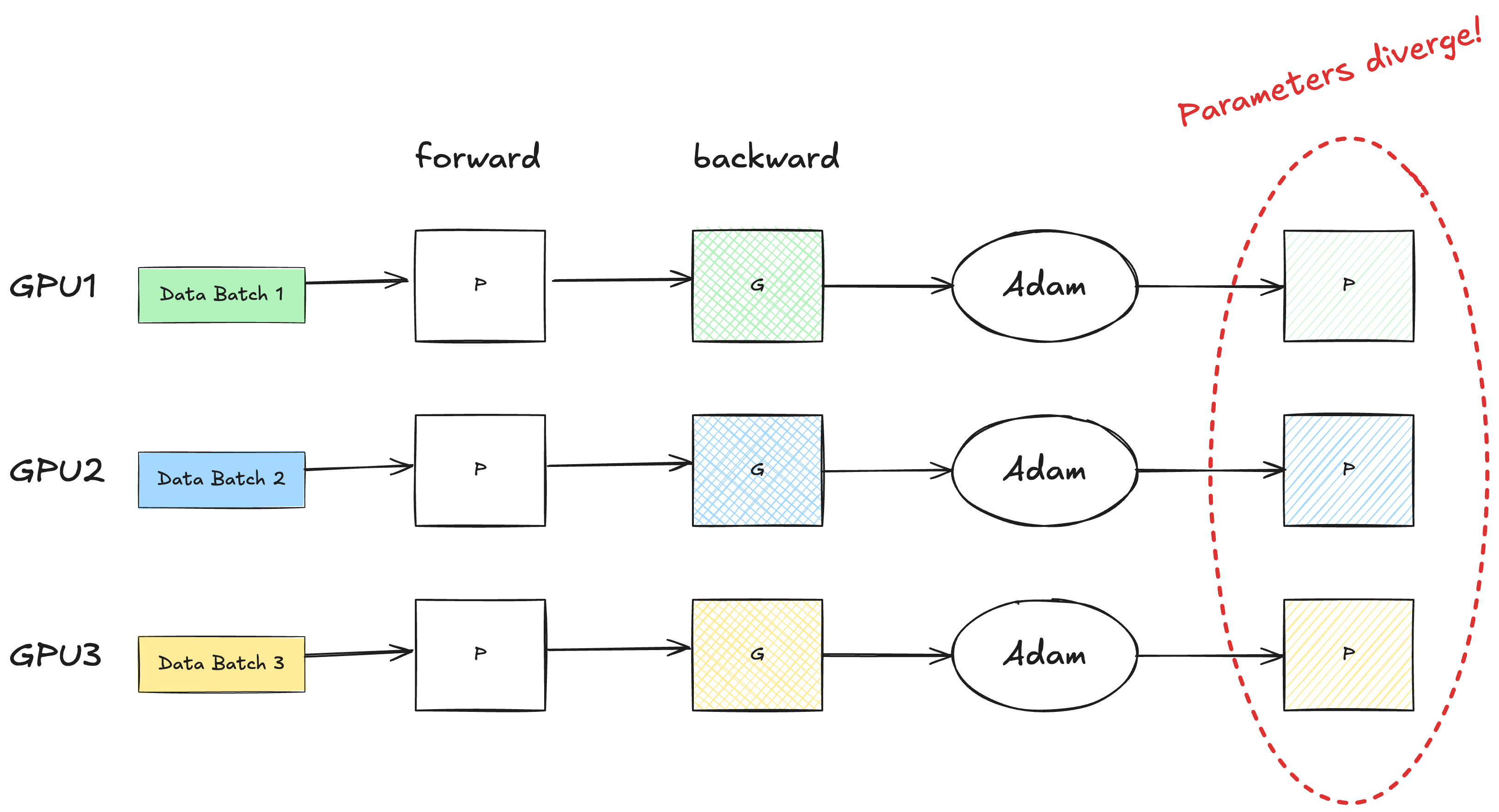
In standard DP, each GPU worker accepts a different input data batch, runs it forward through the network, backpropagates to compute the gradients, and updates the parameters for the next iteration. Because the input data are different, so are the gradients. Without any communication, these gradients would produce different updated parameters, meaning that the model would diverge after one iteration.

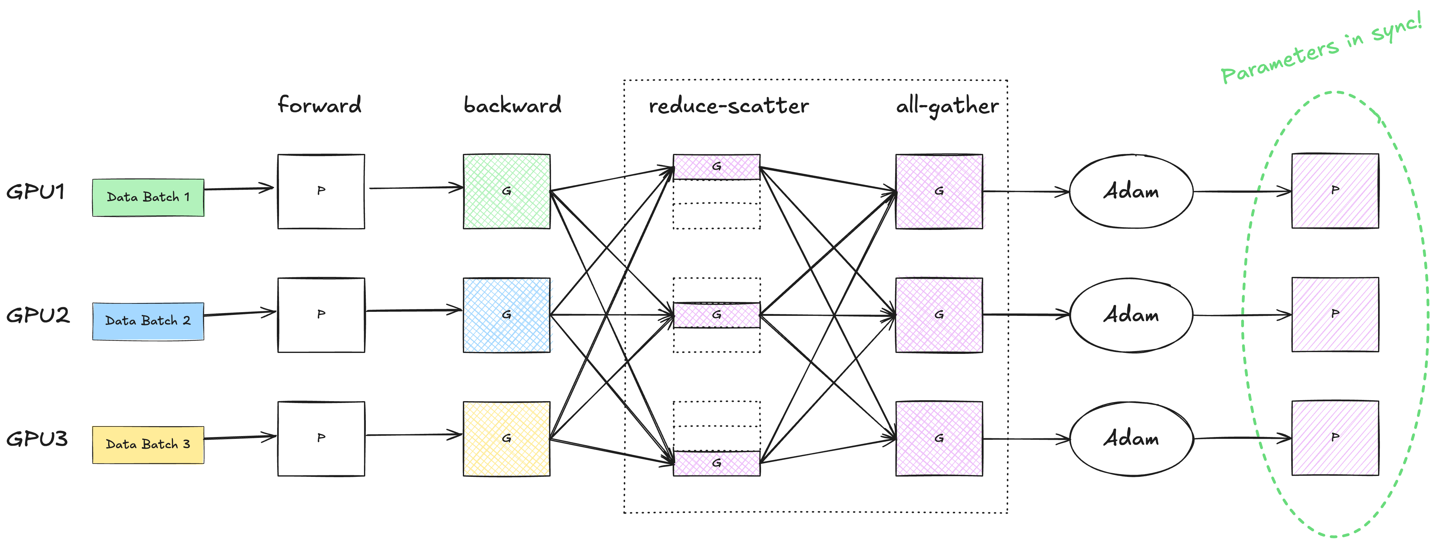
To make sure that the model parameters stay in sync on all GPUs, we need an additional reduction step. Reduction is a fancy word to say “sum the gradients across all GPUs and take the average” (this is oversimplified, as reduction is not limited to summation). The averaged gradients are then sent back to every GPU in the cluster. This way, the gradients, the operator states and the parameters are in sync again.

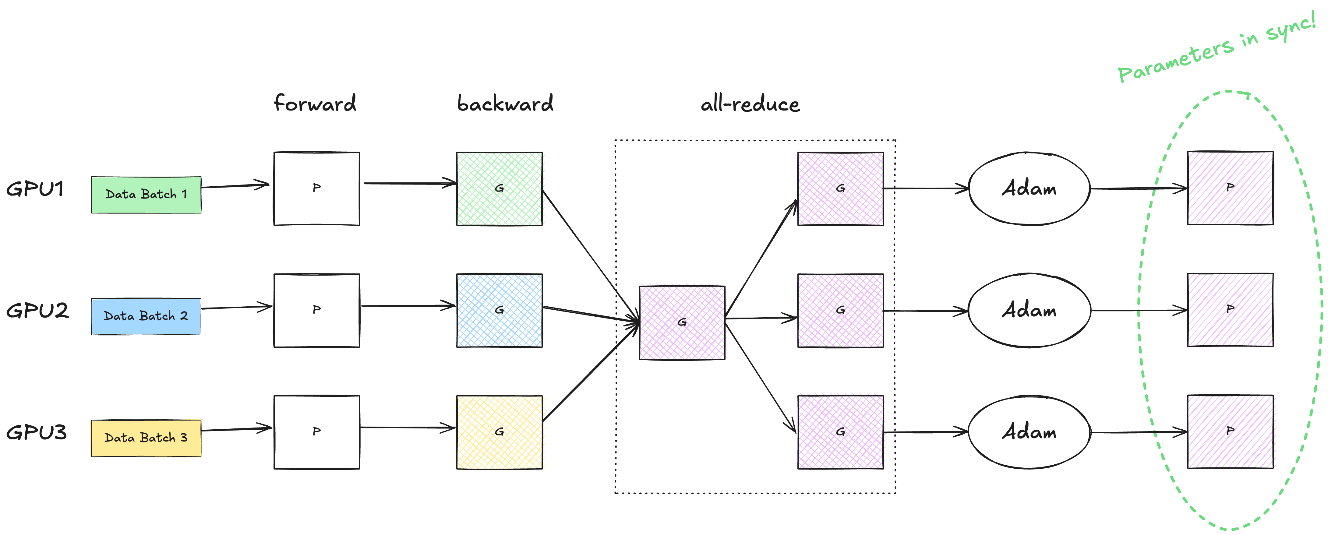
This reduction step can be implemented as an all-reduce via Nvidia’s NCCL. Here, rank refers to the global index of a GPU device among the cluster.

According to the ZeRO paper, state-of-the-art implementation of all-reduce uses a two-step approach, where the first step is a reduce-scatter operation, which reduces different part of the data on different process. The next step is an all-gather operation, where each process gathers the reduced data on all the process.

I’ve attached the charts from the NCCL documentation. You can verify for yourself that an all-reduce is equivalent to a reduce-scatter followed by an all-gather.

For an array of Ψ values, the communication volume of both the reduce-scatter and the all-gather are Ψ elements. Therefore, the standard DP incurs 2Ψ data movement during each training step.

Below shows the complete flow of one training iteration in standard DP.

ZeRO Stage 1 (os)

In ZeRO stage 1, only the optimizer states are partitioned. There is no need to do an immediate all-gather of the gradients after the reduce-scatter step. Instead, we feed the partial gradients into the optimizer, which updates the parameters of its partition. It is these parameter partitions that go through the all-gather step, so that each GPU device can get an identical copy of the full parameters.

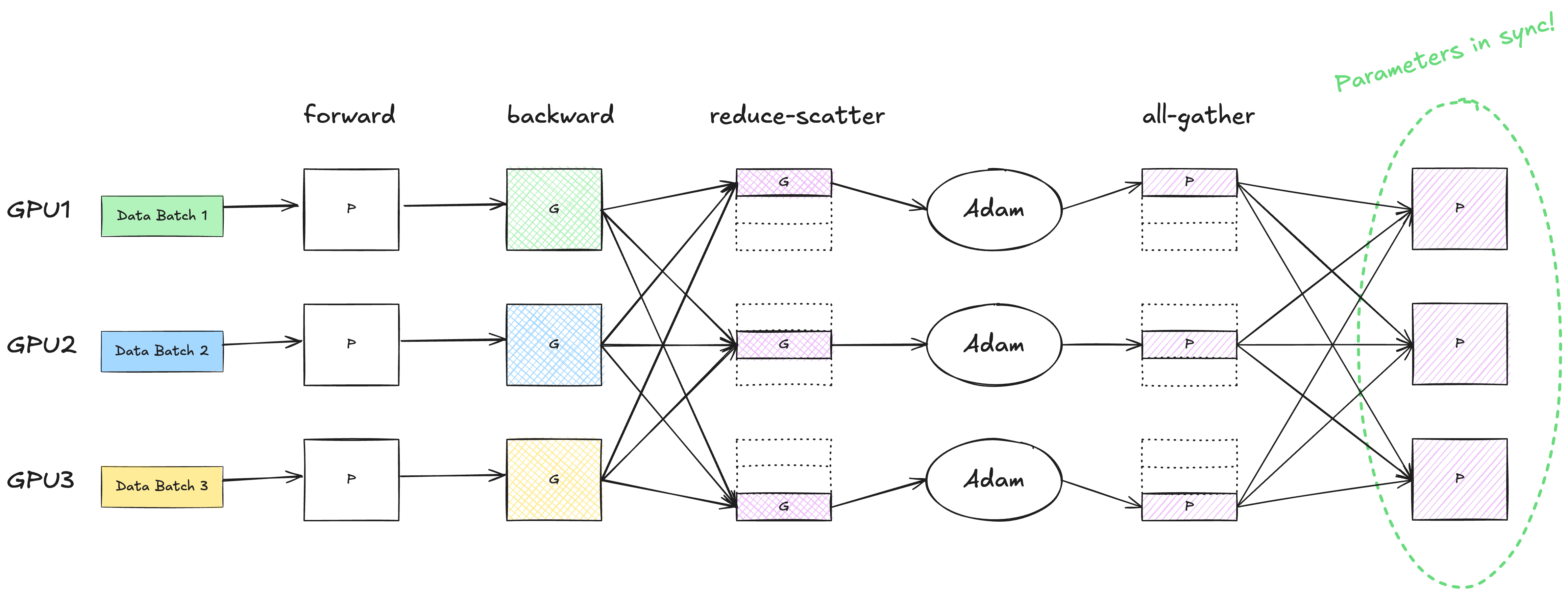
We can see that all stage 1 does is reordering the all-gather step, and applying all-gather on the parameters instead of the gradients. No more or less communication is introduced. Therefore, ZeRO-DP stage 1 has the same communication volume as standard DP does.

ZeRO Stage 2 (os + g)

Stage 2 partitions both the optimizer states and the gradients. Conceptually, this is a natural extension of Stage 1, as the optimizer only needs the gradient partition to work out the rest.

Admittedly, this was the first thing that came to my mind:

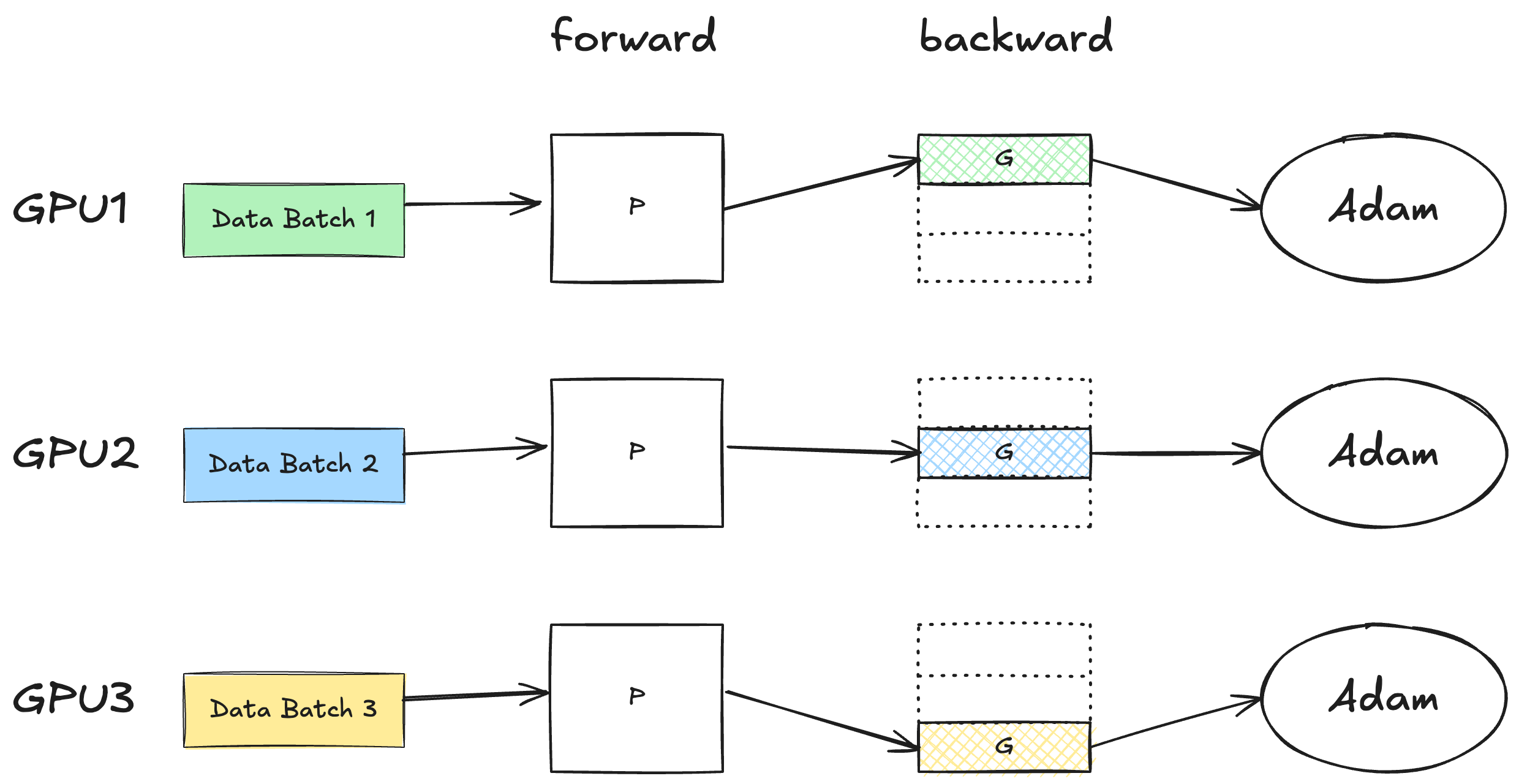
However, this doesn’t work because different GPUs work on different data batches. If during the backward step, gradients not covered by a given GPU worker are masked out, that means we are effectively dropping valuable information for the optimization. In another word, for a given domain to be partitioned, we must wait for all the GPU workers to finish the computation over that domain, before the memory can be released.

Does that mean the GPU workers have to wait for backpropagation to complete? How is this different from Stage 1 and save peak VRAM usage at all?

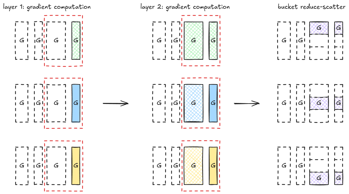
Because each layer is an independent domain for gradient computation, it allows a GPU worker to compute gradients for one layer, perform a reduce-scatter, release vRAM, move on to the next layer, and so on and so forth.

The chart below illustrates the ZeRO stage-2 gradient computation steps for a 4-layer gradient. We can see that the peak vRAM usage during this process is bounded by the max single layer size. The communication volume stays the same, as the total amount of values being exchanged is still Ψ. However, we run the reduce-scatter operation multiple times (which could still hurt performance, as NCCL errors are one of the common reasons to slow down or pause the training).

To make this process more efficient, the paper says that:

we use a bucketization strategy, where we bucketize all the gradients corresponding to a particular partition, and perform reduction on the entire bucket at once.

By now, this should be straightforward to understand: Instead of doing a reduce-scatter immediately after the gradients of a layer is computed, we accumuate them to a pre-allocated bucket, and only trigger the reduce-scatter when this bucket is full.

ZeRO Stage 3 (os + g + p)

Stage 3, being the full form of ZeRO-DP, partitions the parameters as well, on top of the gradients and the optimizer states. Here’s how it works:

1. During the forward pass, a GPU worker needs an all-gather operation to receive the parameters for all the other partitions to compute loss l. Once the forward pass for that specific partiion (or layer) is done, the vRAM can be released. This results in a Ψ communication volume.

2. During the backward pass, a parameter all-gather is carried out again for gradient computation. This results in a Ψ communication volume.

3. Finally, we need a reduce-scatter to average the gradients and scatter them to the GPU workers. This results in a Ψ communication volume.

The total communication volume is 3Ψ, representing a 1.5x amplification compared to the previous two ZeRO stages and standard DP.

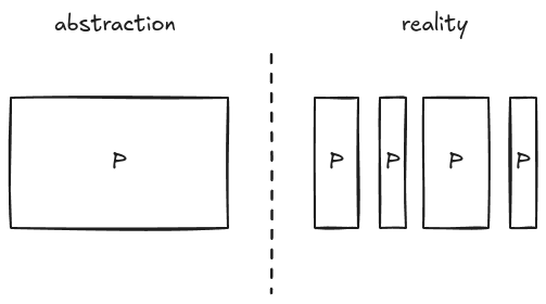
The chart above illustrates the forward and backward passes in ZeRO Stage 3. Again, it’s slightly misleading because: 1) the entire parameter block is all-gathered to a single device, and 2) the entire gradient block is computed before reduce-scatter. In reality, memory from a layer can be released for the next layer as soon as it is processed.

Appendix: Code Walkthrough of ZeRO Stage 2

The first Github PR I found relevant to ZeRO stage 2 is https://github.com/microsoft/DeepSpeed/pull/217, or commit f2ac7ea. It is interesting to look at their initial implementation process and confirm our understanding.

The file to look at is deepspeed/pt/deepspeed_zero_optimizer.py. The terminology here is independent partition gradient, short for ipg. ipg_buffer is the pre-allocated bucket tensor. For simplicity, let’s assume that there is only a single parameter group and a single process group. We will also look at the code path where contiguous_gradients is true (the default).

1. reduce_independent_p_g_buckets_and_remove_grads(self, param, i): This function is registered as a gradient accumulation hook for every parameter participating in the gradient computation. The code path reads as:

   1. (code) If the combined elements in the ipg bucket and the parameter is larger than the bucket size, invoke reduce_ipg_grads() to perform a bucket-wise gradient reduction.

   2. (code) The reduced gradients in the bucket is copied back to the gradient tensor attached to the parameter.

2. reduce_ipg_grads(): The function invokes average_tensor(), copies the reduced gradients to each gradient tensor, and clears the states of the ipg bucket.

3. average_tensor(tensor):

   1. (code) For each param’s gradient in the ipg bucket to be reduced, find its belonging partition id and the gradient offset within the partition (grad_start_offset). This is stored in partition_ids_w_offsets. If you trace back the calling stack, you will find that loop variable i is the index of the parameter group. Just ignore it.

   2. (code) Each tuple in partition_ids_w_offsets roughly corresponds to a region within the ipg bucket to be reduced to a particular rank (i.e. the partition id of the GPU worker). Range merging is possible, provided that they go to the same rank. rank_and_offsets stores a 3-tuple of (reduce destination rank, range begin, range size).

   3. (code) Average the values in the ipg bucket. Then reduce a given bucket range to a specific rank for each record in rank_and_offsets.

Note that it is the regular reduce operation being used, instead of reduce-scatter. Considering that a gradient tensor is relatively small (compared to the entire vRAM space), the implementation reveals that what each GPU worker is really managing is a set of tensors in its partition, as opposed to the notion that the states are horizontally partitioned.